| |
Egwald Mathematics: Optimal Control
The Rocket Car
by
Elmer G. Wiens
Egwald's popular web pages are provided without cost to users.
Follow Elmer Wiens on Twitter:

|
A rocket car runs on rails over a flat plain (Pontryagin et al. 23). Two rocket engines are mounted on the car, one at the front and one at the rear of the car. Firing the rear engine propels the car forward (in a positive direction); firing the front engine propels it backwards (in a negative direction).
From physics I know F = m*a, where F is the force, m is the mass, and a is the acceleration. Assume that the car has mass m = 1. The car's rocket engines provide the force F. Recall that in a given coordinate system, velocity is the rate of change of position with respect to time, and acceleration is the rate of change of velocity with respect to time.
Let x1(t) be the position of the car at time t. Then its velocity x2(t) at time t is the derivative of x1(t) with respect to time t.
1. velocity = x2(t) = dx1(t) / dt
The acceleration of the car at time t, dx2(t)/dt, equals the force F of the rocket engines at time t, denoted by u(t). Firing the rear engine, u(t) > 0, accelerates the car forward; firing the front engine, u(t) < 0, accelerates the car backward.
2. acceleration = dx2(t) / dt = u(t)
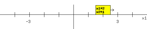
The differential equations, 1) and 2), and the initial conditions or the values of x1 and x2 at the start (t = 0), provide the dynamics of the system. The initial position x1(0) = 2 and initial velocity x2(0) = 1 of the rocket car are shown below. The arrow shows the direction in which the car is moving at the start, depending on the sign of x2(0).
I want to fire the rocket engines, either front or back, in sequence to return the rocket car to the origin x1 = 0, where it is to be at rest x2 = 0, in the least time possible. By controlling u(t) I control the speed and position, the dynamics, of the rocket car. Engineering constraints require that the rockets' force be limited as:
-1 <= u(t) <= 1 with u a piecewise continuous (PWC) function.
So, a value of u(t0) = -.5 means that I am firing the front rocket engine with a force of .5 at time t0. A value of u(t1) = .75 means that I am firing the rear rocket engine with a force of .75 at time t1.
|
|
The optimal (minimum time) firing sequence depends on the rocket car's initial position x1(0) = 2 and initial velocity x2(0) = 1.
Applying Optimal Control Theory to this situation, the optimal firing sequence is:
|
u(t) =
|
-1 : 0 <= t <= 2.58
|
|
1 : 2.58 <= t <= 4.16
|
With the firing sequence above, the rocket car will be at rest at the origin at time t = 4.16.
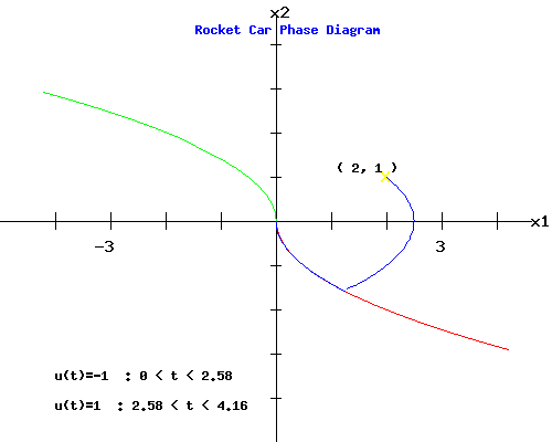
The dynamics of the system are shown in the phase diagram below, showing the time paths of the rocket car's position x1(t) and velocity x2(t) from its initial position and velocity, in response to the optimal firing sequence.
You can change the rocket car's initial situation. Enter new values for x1(0) and x2(0) in the form below the phase diagram. See how the rocket car's start shifts, and how the phase diagram changes after you click Fire Rockets. Try x1(0) = 2.5 and x2(0) = -3, for example.
|
|
The blue arc in the phase diagram above shows the trajectory of the position, x1(t), and velocity, x2(t), in response to the firing sequence encoded in u(t). The green and red arcs show time paths of position and velocity that travel directly to the origin.
Set x1(0) = -2 and x2(0) = 2 in the form above, and click Fire Rockets. If you do this, you will see that the blue arc proceeds directly to the origin along the green trajectory. What happens if you set x1(0) = 2 and x2(0) = -2?
|
Matlab Program to generate Rocket Car Phase Diagram as Figure 1.
|
Pontryagin Maximum Principle
Optimal control problems can be solved using the Pontryagin Maximum Principle.
Start by setting up the problem in its matrix from:
|
|
A =
|
| 0 1 |
| 0 0 |
|
B = |
| 0 |
| 1 |
|
|
|
Let the symbol t represent terminal time,
and the symbol T represent the transpose of a vector.
The trajectory of the state variables x(t) = (x1(t), x2(t))T is described by:
dx(t) / dt = A * x(t) + B * u(t)
x(0) = (x1(0), x2(0))T
x(t) = (0, 0)T
Introduce a new vector of variables p(t) = (p1(t), p2(t))T called the adjoint (co-state) variables, one for each state variable; the "normality indicator" µ0 >= 0, which is the Lagrange multiplier on the objective function Î(t) = t; and, a vector of Lagrange Multipliers µ = (µ1, µ2)T,
Minimum Time Optimal Control Problem
The Maximum Principle is based on the Pre-Hamiltonian function, which in this minimum time problem takes on the form (Loewen, Lecture Notes):
H(t, x(t), p(t), u(t)) = p(t)T * (A * x(t) + B * u(t))
If the control-state pair (u*, x*) represent the optimal control and trajectory, define the function:
h*(t) = H(t, x*, p, u*).
|
| a. Adjoint equations: |
dh*(t) / dt = dH(t, x*, p, u*) / dt
dHT / dx = -dp(t) / dt = AT * p(t) |
| b. State equations: | dHT / dp = dx(t) / dt = A * x*(t) + B * u*(t) |
| c. Maximum Condition: | dH / du = p(t)T * B -> u(t) = sgn(p(t)T * B) |
|
d. Transversality Conditions:
|
(h*(t), -p1(t), -p2(t)T = (µ0, µ1, µ2)T
|
| e. Nontriviality: | p(t) is not equal to 0 for all t. |
|
|
In the rocket car problem the state variables have both initial and terminal conditions. Therefore, the adjoint differential equations for p(t) and the constants, (µ1, µ2), are not necessary. However, I introduce them and I solve them to illustrate their function in problems where some of the initial and terminal conditions for the state variables are unavailable. Since dh*(t) / dt = 0, H does not depend explicitly on t, H(t, x*, p, u*) is constant on 0 <= t <= t.
State Variables:
Let u(0) = u1 be the value of u(t) at the start. Solving the state differential equations yields :
|
|
x1(t) = x1(0) + x2(0) * t + u1 * (1/2) *t^2
x2(t) = x2(0) + u1 * t
To find the trajectories that reach the origin,
set x1(0) = 0 and x2(0) = 0 above yielding:
x1(t) = u1 * (1/2) * t^2
x2(t) = u1 * t
|
|
|
In the phase diagram above, the trajectory of x(t) = (x1(t), x2(t))T for u1 = 1 is the red arc, while the trajectory for u1 = -1 is the green arc. (Run time backward from t = 0 to get the trajectories that enter the origin.)
|
|
Adjoint Variables:
Solving the adjoint differential equations yields:
|
|
p1(t) = p1(t)
p2(t) = p1(t) * (t - t) + p2(t)
|
|
|
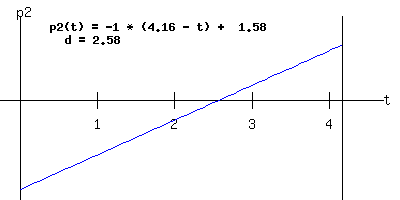
From the maximum condition, u(t) = sgn(p(t)T * B) = sgn(p2(t)). If I graph p2(t) as a function of t, u(t) switches from u1 to -u1, when p2(t) = 0. Call this switch time t = d, i.e. p2(d) = 0.
p2(d) = p1(t) * (t - d) + p2(t) = 0
--> d = t + p2(t) / p1(t)
In the example with initial position x1(0) = 2 and initial velocity x2(0) = 1, the graph of the p2(t) curve below has a switch time of d = 2.58.
|
|
Terminal and Switch Time:
So, how did I obtain the terminal time, t = 4.16, and the switch time d = 2.58. If the starting values, x(0) = (x1(0), x2(0))T, lie on one of the trajectories that enter the origin, then d = 0, and t = abs(x2(0)). (Try a few trajectories to convince yourself.)
Otherwise, I need to know either:
i) the switch time d, allowing me to compute the switch coordinates x(d), where the trajectory starting from x(0) intersects one of the trajectories that enter the origin, yielding the terminal time, or
ii) the switch position and velocity, x(d), yielding the switch time d and terminal time t.
The state differential equations are:
dx(t) / dt = A * x(t) + B * u1
0 <= t <= d, x(0) and x(d) given
dx(t) / dt = A * x(t) + B * u2
d <= t <= t, x(d) and x(t) = (0,0)T given, and u2 = - u1.
The equations of motion for d <= t <= t are:
x1(t)= x1(0) - u1 * d^2 + t * x2(0) + 2 * u1 * t * d - (1/2) * u1 * t^2
x2(t) = x2(0) + 2 * u1 * d - u1 * t
To find d and t, set x(t) = (0, 0)T in the last pair of equations, and solve for d and t yielding:
d = ((-1/2) * u1) * x2(0) + (1/2) * t
t = x2(0) + sqrt(2) * sqrt(x2(0)^2 + 2 * x1(0)) if u1 = -1;
t = - x2(0) + sqrt(2) * sqrt(x2(0)^2 - 2 * x1(0)) if u1 = 1;
The terminal values of the adjoint functions are:
p1(t) = u1 = -1,
p2(t) = p1(t) * (d - t) = 1.58.
|
|
Switch Coordinates:
The switch coordinates are x1(d) = 1.25, x2(d) = -1.58. The position of the rocket car at the switch time appears below:
|
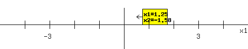
|
After the switch time, the
rear rocket engine is fired for 1.58 time units, bringing the rocket car to rest at the origin at time t = t = 4.16.
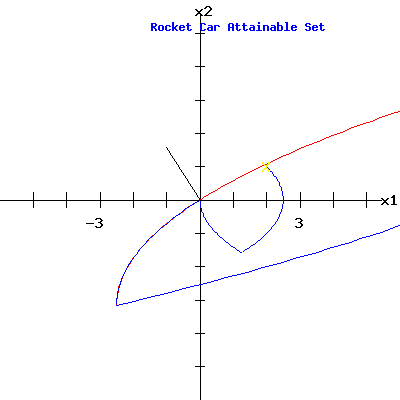
Attainable Set:
The attainable set, Å, consists of those points (x1,x2) that can be reached in time t = 4.16 from the initial coordinates (2, 1) using firing sequence controls u(t) that satisfy the engineering constraints:
U = {u(t): u is a PWC function on [0, 4.16], and -1 <= u(t) <= 1}
Control functions u(t) that are members of U are called admissible controls.
Formally,
Å(t, x(0), U) = {x(t): x'(t) = A*x(t) + B*u(t), x(0) = (x1(0),x2(0))T, u(t) a function in U}
Extremal Trajectories:
Trajectories, x(t), that satisfy conditions a, b, c, and e, of the Pontryagin Maximum Principle are called extremal trajectories. Extremal trajectories always lie on the boundary of the attainable set Å.
|
|
In our minimum time problem, with the origin as a terminal condition of the trajectories, the vector of adjoint variables at terminal time, shown in black:
p(t) = (p1(t), p(t)) = (-1, 1.58)
is perpendicular to the boundary of the attainable set Å at the origin.
Matlab Program to generate Rocket Car Attainable Set as Figure 2.
Controllability:
The system of differential equations that governs the trajectory of the state vector x(t):
dx(t) / dt = A * x(t) + B * u(t)
can be classified as a linear autonomous system, because A and B are constant matrices. A linear autonomous system is called controllable if the state vector, x(t), can be guided to a given target set T(t) using some admissible control function u(t).
Controllability Matrix:
For a linear autonomous system, with matrices A and B, the controllability (Pontryagin et al. 116) matrix for a system with two state variables is:
C = [ B | A * B]
For the Rocket Car:
|
|
|
|
The rank of C is 2, which equals the number of state variables; the matrix A has two eigenvalues = 0. Therefore, for any initial state x(0) = (x1(0), x2(0))T an admissible control function, u(t), exists that will steer the evolution of the trajectory of state variables, x(t), to the target set, T = (0, 0)T.
|
Works Cited and Consulted
-
Intriligator, Michael D. Mathematical Optimization and Economic Theory. Englewood Cliffs: Prentice-Hall, 1971.
-
Lewis, Frank L. Optimal Control. New York: Wiley, 1986.
-
Loewen, Philip D. Math 403 Lecture Notes. Department of Mathematics, University of British Columbia. 4 Apr 2003. http://www.math.ubc.ca/~loew/m403/.
-
Macki, Jack and Aaron Strauss. Introduction to Optimal Control. New York: Springer-Verlag, 1982.
-
Pontryagin, L. S., V. G. Boltyanskii, R. V. Gamkrelidze, and E. F. Mishchenko. The Mathematical Theory of Optimal Processes. Trans. K.N. Trirogoff. New York: Wiley, 1962.
|
|