| |
Egwald Mathematics: Optimal Control
Linear-Quadratic Regulator
by
Elmer G. Wiens
Egwald's popular web pages are provided without cost to users.
Follow Elmer Wiens on Twitter:

|
Minimum Effort Servomechanism:
Suppose I can influence the evolution of a vector of n state variables x(t) = (x1(t), ..., xn(t))T with a vector of control variables u(t) = (u1(t), ..., ur(t))T (here the symbol "T" represents the transpose of a vector) as given by:
dx / dt = A * x(t) + B * u(t)
where A is an n x n matrix and B is an n x r matrix.
At each instance of time t, I incur a cost that depends on the values of the state variables and control variables at that time. I want to minimize the total costs over a relevant planning interval of time. Formally, the problem is as follows:
Given symmetric, nonnegative, semidefinite matrices D, (nxn), M, (nxn), and R, (nxr), and a planning interval [t0, t], choose a piecewise smooth function u from [t0, t] to Rr so as to minimize the sum of the terminal cost and running cost given by:
|
|
min J[u] = x(t)T*D*x(t) +
 (x(t)T*M*x(t) + x(t)T*R*u(t) + u(t)T*RT*x(t) + u(t)T*u(t) ) dt
dx / dt = A * x(t) + B * u(t)
x(t0) = x0
Because the problem above has no constraint on x(t), it is a free final state problem, with a feedback optimal control.
With a fixed final state constraint of the form x(t) = xt, the optimal control will be an open-loop control.
|
|
Finite Horizon Time Problems
Matrix Ricatti Equation:
With a finite planning horizon, t <  , linear-quadratic optimal control problems are solved by finding the symmetric n x n matrix K = K(t) that satisfies the Matrix Ricatti Equation (MRE): , linear-quadratic optimal control problems are solved by finding the symmetric n x n matrix K = K(t) that satisfies the Matrix Ricatti Equation (MRE):
dK / dt + AT * K + K * A - (K * B + R) * (BT* K + RT) + M = 0, K(t) = D
Optimal Closed Loop (Feedback) Control:
If K(t) solves MRE, then the optimal closed loop control is:
u*(t) = - (BT * K + RT) * x(t)
Evolution of the Optimal State Variables:
dx(t) / dt = A * x(t) - B * (BT * K + RT) * x(t)
= ( A - B * (BT * K + RT) ) * x(t)
Solving these differential equations with the initial conditions x(t0) = x0 yields x = (x1, ..., xn)T as a function of time and x0.
|
|
Example 1 (Pinch 167):
Consider a system with two state variables, and A = 0, B = I, D = I, M = 0, and R = 0, where I is the identity matrix. Then
dx1 / dt = u1(t)
dx2 / dt = u2(t)
min J[u] = x12(3) + x22(3) +
 (u12(s) + u22(s) ) ds
1. MRE:
dK / dt = K * K, K(3) = D = I
|
|
|
|
2. Optimal Closed Loop Control:
u*(t) = - BT * K * x(t)
3. MRE Differential Equations:
dk1 / dt = k12 + k32 k1(3) = 1
dk3 / dt = k3 * (k1 + k2) k3(3) = 0
dk2 / dt = k32 + k22 k2(3) = 1
4. Integrating the differential equations:
k3 = 0
k1 = 1 / (4 - t)
k2 = 1 / (4 - t)
K = (1 / (4 - t)) * I
5. Optimal control in feedback form:
u(t) = - BT * K * x(t) = (1 / (t - 4)) * x(t)
6. Optimal state variable trajectory:
dx(t) /dt = u(t) = (1 / (t - 4)) * x(t)
which integrates to yield:
x(t) = - ((t - 4) / 4) * x(0)
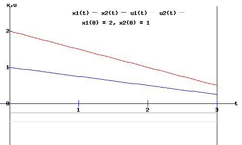
7. Optimal control as a function of time and x(0):
u(t) = - 1/4 * x(0)
The time paths of the state variables, x(t), and the control variables, u(t), are shown in the diagram below.
|
|
Infinite Time Horizon Problems
If the planning horizon extends to infinity, then K(t) must remain finite as t -> , requiring dK / dt = 0. To find the equilibrium K(t) = Ke, solve the Algebraic (Steady-State) Ricatti Equation (ARE):
Algebraic (Steady-State) Ricatti Equation (ARE):
AT * K + K * A - (K * B + R) * (BT* K + RT) + M = 0
Optimal Feedback Control Law:
u*(x(t)) = - (BT * K + RT) * x*(t)
Minimum Cost Solution:
J[u*] = x(0)T * K * x(0)
Example 2 (Hocking 124-25):
Consider the Rocket-Car problem with costs that depend both on position, x1(t), and energy expended, u(t).
dx1 / dt = x2(t)
dx2 / dt = u(t)
min J[u] = (4 * x1(t) * x1(t) + u(t) * u(t) ) dt
with t0 = 0, and
|
|
A =
|
| 0 1 |
| 0 0 |
|
B =
|
| 0 |
| 1 |
|
M =
|
| 4 0 |
| 0 0 |
|
D = | 0 | R = | 0 |
|
|
|
1. MRE Differential Equations:
dk1 / dt = k32 - 4 k1(t) = 0
dk3 / dt = k2 * k3 - k1 k3(t) = 0
dk2 / dt = k22 - 2 * k3 k2(t) = 0
2. ARE Solution:
k3 = 2, k1 = +/- 4, k2 = +/- 2
For K to be a positive definite matrix:
|
|
|
|
3. Optimal Feedback Control Law:
u*(x(t)) = - (BT * K) * x*(t) = (-2, -2) * (x1(t), x2(t))T
4. Optimal Evolution of State Variables:
dx / dt = A * x(t) + B * u*(x(t))
|
|
dx / dt =
|
| 0 1 |
| 0 0 |
|
* (x1(t), x2(t))T +
|
| 0 0 |
| -2 -2 |
|
* (x1(t), x2(t))T
|
|
dx / dt =
|
| 0 1 |
| -2 -2 |
|
* (x1(t), x2(t))T
|
= Â * x(t)
|
|
|
5. Optimal Trajectories of the State Variables:
The autonomous linear differential equation above has the solution:
x*(t) = expm(Â * t) * x(0),
where expm( * t) is the matrix exponential, e * t. The explicit solution is:
|
|
x*(t) =
|
| exp(-t)*cos(t)+exp(-t)*sin(t) exp(-t)*sin(t) |
| -2*exp(-t)*sin(t) exp(-t)*cos(t)-exp(-t)*sin(t) |
|
* x(0)
|
|
|
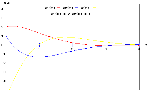
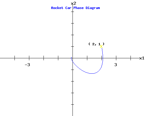
6. Minimum Cost Solution with (x1(0), x2(0)) = ( 2, 1 ):
J[u*] = x(0)T * K * x(0) = 26
In the diagrams below, you can see the trajectories of the state and control variables plotted as a function of time, and the phase diagram of x2(t) plotted against x1(t), with an initial position of (x1(0), x2(0)) = ( 2, 1 ).
You can change the rocket car's initial situation by entering new values for x1(0) and x2(0) in the form below the phase diagram. See how the trajectories shift, and how the phase diagram changes after you click Fire Rockets. Try x1(0) = -2.5 and x2(0) = -3, for example. When u(t) is positive, the rear rocket is firing; when u(t) is negative, the front rocket is firing. (Go to the Rocket-Car page for a full description of this optimal control problem).
|
Works Cited and Consulted
-
Hocking, Leslie M. Optimal Control: An Introduction to the Theory with Applications. Oxford: Clarendon, 1991.
-
Intriligator, Michael D. Mathematical Optimization and Economic Theory. Englewood Cliffs: Prentice-Hall, 1971.
-
Lewis, Frank L. Optimal Control. New York: Wiley, 1986.
-
Loewen, Philip D. Math 403 Lecture Notes. Department of Mathematics, University of British Columbia. 4 Apr 2003. http://www.math.ubc.ca/~loew/m403/.
-
Pinch, Enid R. Optimal Control and the Calculus of Variations. Oxford: Oxford UP, 1993.
|
|