| |
Egwald Mathematics: Optimal Control
The Linearized Pendulum
by
Elmer G. Wiens
Egwald's popular web pages are provided without cost to users.
Follow Elmer Wiens on Twitter:

|
The motion of a pendulum in a vertical plane can be described by the differential equation:
L * d2Ø(t) / dt2 + g * sin(Ø(t)) - u(t) = 0
where Ø(t) is its angular displacement in degrees from the vertical at time t, L is the length of the cord attached to the ball of the pendulum, g is the force of gravity, and u(t) is the control variable (forcing term) at time t. When u(t) > 0, the force pushes the ball of the pendulum to the right; when u(t) < 0, the force pushes the ball of the pendulum to the left.
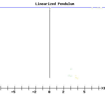
The objective is to use the control u(t) to bring the pendulum to rest as quickly as possible. The intuitive idea is to push or pull (green arrow) against the movement (red arrow) of the pendulum, resisting its momentum. However, the minimum time solution pushes with the momentum for short periods of time. The animated image below shows how this works. (Wait a few seconds and it will repeat.)
For small values of Ø(t), sin(Ø(t)) is approximately Ø(t). Let x1(t) = Ø(t), the angular displacement of the pendulum, and dx1(t) /dt = x2(t), the angular velocity of the pendulum.
The diagram below depicts the position of the pendulum with an initial angular displacement of 4, and angular velocity of 4. The red arrow points in the direction the pendulum swings; the green arrow points in the direction the forcing term pushes.
|
|
By choosing the units of all variables appropriately, the system of differential equations that governs the movement of the pendulum is:
|
| ( * ) |
dx1 / dt = x2(t)
dx2 / dt = -x1(t) + u(t)
with -1 <= u(t) <= 1
|
|
|
The constraints on u(t) indicate that the force applied to the ball of the pendulum cannot exceed its mass in magnitude, i.e.
u = acceleration = F / m. The balls acceleration, dx2 / dt, equals the sum of the force of gravity, -x1(t), plus the force of the control variable, u(t).
The solution to this problem appears in many textbooks (Pontryagin et al. 27) or (Hsu and Meyer 552), and is called "the time-optimal control of an oscillating plant with no damping and with a single input" in Engineering literature, or the "Harmonic Oscillator" in Physics.
First, I will discuss the well known solution to the system of differential equations ( * ), and then I will use Pontryagin's Maximum Principle to analyze the interaction of the state variables and adjoint variables.
From ( * ),
(x1 - u)*dx1 / dt + x2 * dx2 / dt = 0
Integrating with respect to time while holding u constant,
(x1 - u )2 + x22 = d2
a circle of radius d and center u, where u is +1 or -1.
The trajectory of the state variables x(t) = (x1(t),x2(t)) will be arcs with equations:
(x1 - u) = d * cos(t + ß)
x2 = -d * sin(t + ß)
with x(t) traversing the circles in a clockwise direction as t increases, and d and ß constants that determine the appropriate circle.
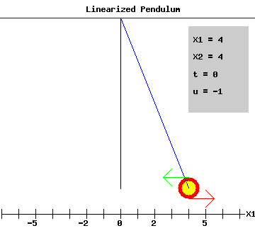
The optimal trajectory of x(t) along with the setting of the forcing term u(t) is shown in the phase diagram below, with (x1(0), x2(0)) = (4, 4). The switching points for u(t) are marked with a * in yellow. The switching points occur where the trajectory of x(t) intersects a semicircle of radius one centered at an odd number. When u(t) = -1, the relevant "switching semicircles" are the negative branch; when u(t) = 1, the relevant "switching semicircles" are the positive branch. For x(t) above the "switching semicircles," optimal controls use u(t) = -1; for x(t) below the "switching semicircles," optimal controls use u(t) = 1. The number of switches in an optimal trajectory depends on the distance between the initial point and the origin. The short arcs in pink show the regions where the optimal forcing term u(t) pushes with the momentum of the pendulum.
|
|
For this example with x(0) = (x1(0), x2(0)) = (4, 4), the switching times and switching points appear in the following table:
|
|
Time
|
x1(s)
|
x2(s)
|
u(s)
|
0 | 4 | 4 | -1 |
0.82 | 5.33 | -0.94 | 1 |
3.96 | -3.33 | 0.94 | -1 |
7.11 | 1.33 | -0.94 | 1 |
9.02 | 0 | 0 | 1 |
|
|
You can change the pendulum's initial situation. Enter new values for x1(0) and x2(0) in the form below. See how the pendulum's start shifts, and how the phase diagram and the graphs of the adjoint variables below change after you click "Swing Pendulum." Try x1(0) = -4.4 and x2(0) = -4.4, for example.
|
Matlab Program to generate the Linear Pendulum Phase Diagram as Figure 1.
|
Pontryagin Maximum Principle
Optimal control problems can be solved using the Pontryagin Maximum Principle.
Start by setting up the problem in its matrix from:
|
|
A =
|
| 0 1 |
| -1 0 |
|
B = |
| 0 |
| 1 |
|
|
|
Let the symbol t represent terminal time,
and the symbol T represent the transpose of a vector.
The trajectory of the state variables x(t) = (x1(t), x2(t))T is described by:
dx(t) / dt = A * x(t) + B * u(t)
x(0) = (x1(0), x2(0))T
x(t) = (0, 0)T
Introduce a new vector of variables p(t) = (p1(t), p2(t))T called the adjoint (co-state) variables, one for each state variable; the "normality indicator" µ0 >= 0, which is the Lagrange multiplier on the objective function Î(t) = t; and, a vector of Lagrange Multipliers µ = (µ1, µ2)T,
Minimum Time Optimal Control Problem
The Maximum Principle is based on the Pre-Hamiltonian function, which in this minimum time problem takes on the form (Loewen, Lecture Notes):
H(t, x(t), p(t), u(t)) = p(t)T * (A * x(t) + B * u(t))
If the control-state pair (u*, x*) represent the optimal control and trajectory, define the function:
h*(t) = H(t, x*, p, u*).
|
| a. Adjoint equations: |
dh*(t) / dt = dH(t, x*, p, u*) / dt
dHT / dx = -dp(t) / dt = AT * p(t) |
| b. State equations: | dHT / dp = dx(t) / dt = A * x*(t) + B * u*(t) |
| c. Maximum Condition: | dH / du = p(t)T * B -> u(t) = sgn(p(t)T * B) |
|
d. Transversality Conditions:
|
(h*(t), -p1(t), -p2(t)T = (µ0, µ1, µ2)T
|
| e. Nontriviality: | p(t) is not equal to 0 for all t. |
|
|
Since dh*(t) / dt = 0, H does not depend explicitly on t, H(t, x*, p, u*) is constant on 0 <= t <= t. In the linearized pendulum problem, the state variables have both initial and terminal conditions. Therefore, the adjoint differential equations for p(t) and the constants, (µ1, µ2), are not necessary. Moreover, since the value of the end point of p(t), p(t) = (p1(t, p2(t))T varies with x(0)= (x1(0),x2(0))T, p(t) also varies. However, I can construct solutions using the control law, u(t) = sgn(p(t)T * B) by systematically varying p(t) until I get a trajectory for x(t) that reaches the origin (0 ,0)T.
Adjoint Variables:
The system of equations that governs the adjoint variables is:
|
|
dp1 / dt = p2(t)
dp2 / dt = -p1(t)
|
|
implying that:
dp12(t) / dt2 + p1(t) = 0
with the solution:
|
|
p1(t) = - g * cos(t + Õ)
p2(t) = g * sin(t + Õ)
|
|
|
for appropriate g and Õ.
Control Variable and Maximum Condition
The maximum condition implies that u(t) = sgn(p(t)T * B), so
u(t) = sgn(p2(t)) = sgn(g * sin(t + Õ))
Since p(t) is scale invariant, I can set g to be + or -1. So, u(t) = sgn(g * sin(t + Õ)) implies u is piecewise continuous with values of +1 or -1 and switches when t + Õ = k*pi.
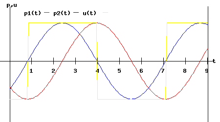
The following diagram shows the interaction of the adjoint and control variables.
|
|
The control variable u(t) jumps from -1 to +1, or from +1 to -1 whenever the graph of p2(t) switches signs. These times and points are called switching times s which occur at time,
0.82, 3.96, 7.11, and switching points,
(5.33, -0.94), (-3.33, 0.94), (1.33, -0.94),
respectively.
Matlab Program to generate the Linear Pendulum: Adjoint and Control Variable diagram as Figure 2.
State Variables:
The general solution of the state differential equations is determined as follows (Huntley and Johnson 45).
|
|
Given a fixed point x(s) = (x1(s), x2(s))T at time t = s,
the state variables values at time t >= s are:
|
|
x(t) =
|
| cos(t-s), sin(t-s) |
| -sin(t-s), cos(t-s) |
|
* x(s) +
|
| sin(t-s), 1-cos(t-s) |
| -1+cos(t-s), sin(t-s) |
|
* B * u
|
|
|
Since B = (0, 1)T, the equations for the components of x(t) are:
x1(t) = cos(t-s)*x1(s) + sin(t-s)*x2(s) + u - u*cos(t-s)
x2(t) = -sin(t-s)*x1(s) + cos(t-s)*x2(s) + u*sin(t-s)
where u is determined by the value of the switching variable p2(t). At the initial time (t = 0) s = 0, so x(t) starts at x(0). The trajectory of x(t) proceeds, with u changing sign and x(s) being redefined at each switching point.
|
|
|
|
|
|
|
Works Cited and Consulted
-
Huntley, Ian and R. M. Johnson. Linear and Nonlinear Differential Equations. New York: Wiley, 1983.
-
Hsu, Jay C. and Andrew U. Meyer. Modern Control Principles and Applications. New York: McGraw-Hill, 1968.
-
Intriligator, Michael D. Mathematical Optimization and Economic Theory. Englewood Cliffs: Prentice-Hall, 1971.
-
Lewis, Frank L. Optimal Control. New York: Wiley, 1986.
-
Loewen, Philip D. Math 403 Lecture Notes. Department of Mathematics, University of British Columbia. 4 Apr 2003. http://www.math.ubc.ca/~loew/m403/.
-
Macki, Jack and Aaron Strauss. Introduction to Optimal Control. New York: Springer-Verlag, 1982.
-
Pontryagin, L. S., V. G. Boltyanskii, R. V. Gamkrelidze, and E. F. Mishchenko. The Mathematical Theory of Optimal Processes. Trans. K.N. Trirogoff. New York: Wiley, 1962.
|
|