| |
Egwald Mathematics: Optimal Control
Intercept Missile
by
Elmer G. Wiens
Egwald's popular web pages are provided without cost to users.
Follow Elmer Wiens on Twitter:

|
A scud missile passes directly overhead. The objective is to destroy the scud missile with a shoulder mounted rocket.
The rocket with mass m fires with a constant thrust of F. Since force = mass times acceleration, F = m * a, solving for the variable a yields the thrust acceleration:
a = F / m
The variable under my control is the thrust angle (firing angle), w, the angle of the rocket with respect to the horizon at firing time, t = 0.
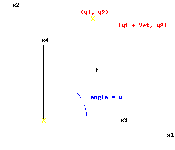
I stand at the origin of the coordinate system. After I fire the rocket, at time t > 0, the position of the intercept rocket is x(t) = (x1(t), x2(t))T (the symbol T represents the transpose of a vector), the rocket's horizontal velocity is x3(t), and vertical velocity is x4(t).
Initially, the position of the scud is y(0) = (y1(0), y2(0))T, and its velocity is V.
At time t, the position of the scud missile will be y(t) = (y1(t), y2(t))T.
The state variables describing the motion of the intercept rocket, x1(t), x2(t), x3(t) x4(t), and the scud missile, y1(t), y2(t), are indicated in the following diagram:
|
|
The evolution of the trajectory of the intercept rocket, and scud missile are described by the following nonlinear system of equations (the symbol t represents terminal time):
|
|
Equations of Motion
|
|
dx / dt = f(t, x(t), w(t))
|
dx1 / dt = x3(t) = f1(t, x(t), w(t))
dx2 / dt = x4(t) = f2(t, x(t), w(t))
dx3 / dt = a * cos(w) = f3(t, x(t), w(t))
dx4 / dt = a * sin(w) = f4(t, x(t), w(t))
|
|
y(t) = g(t, y(t))
|
y1(t) = y1(0) + V * t = g1(t, y(t))
y2(t) = y2(0) = g2(t, y(t))
|
|
At terminal time t, the rocket intercepts the scud missile:
x1(t) = y1(t)
x2(t) = y2(t)
|
|
|
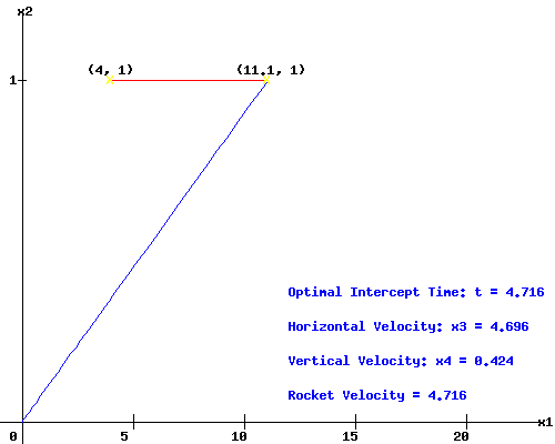
To make the problem tractable, I assume that a = 1, y(0) = (4, 1), and .75 <= V <= 2.75. Thus, the thrust of the rocket engine of the intercept rocket equals its mass, and the scud missile flies at a constant height with a constant velocity.
I want to destroy the (advanced) scud missile as quickly as possible, to prevent it from taking any evasive maneuvers. The optimal control, minimum time, intercept trajectory given the scud missile has velocity V = 1.5 is shown below, if I fire the intercept rocket at the optimal angle w = 5.16 degrees or 0.09 radians:
|
|
You can change the velocity, V, of the scud missile to see how the optimal intercept trajectory varies with V.
|
|
Pontryagin Maximum Principle
Optimal control problems can be solved using the Pontryagin Maximum Principle.
Introduce variables:
p(t) = (p1(t), p2(t), p3(t), p4(t))T
called the adjoint (co-state) variables, one for each state variable;
the "normality indicator" µ0 >= 0, the Lagrange multiplier on the objective function Î(t) = t;
and, a vector of Lagrange Multipliers:
µ = (µ1, µ2, µ3, µ4)T.
Minimum Time Optimal Control Problem
The Maximum Principle is based on the Pre-Hamiltonian function, which in this minimum time problem takes on the form (Loewen, Lecture Notes):
H(t, x(t), p(t), w(t)) = p(t)T * f(t, x(t), w(t)) = p1 * x3 + p2 * x4 + p3 * cos(w) + p4 * sin(w)
If the control-state pair (w*, x*) represent the optimal control and trajectory, define the function:
h*(t) = H(t, x*, p, w*).
|
| a. Adjoint equations: |
dh*(t) / dt = dH(t, x*, p, w*) / dt
dHT / dx = -dp(t) / dt = (0, 0, p1(t), p2(t))T |
| b. State equations: | dHT / dp = dx(t) / dt = f(t, x*(t), w*(t)) |
| c. Maximum Condition: | dH / dw = -p3(t) * sin(w*) + p4(t) * cos(w*) = 0
-> tan(w*) = p4(t) / p3(t)
|
|
d. Transversality Conditions:
|
h*(t) = µ0 * Ît(t) - µ1 * g1t(t) = µ0 - µ1 * V
(-p1(t), -p2(t), -p3(t), -p4(t))T = (µ1, µ2, 0, 0)T
|
| e. Nontriviality: | p(t) and the vector (µ0, µ) are not both 0. |
|
|
Since x3(t) and x4(t) are free variables,
(-p3(t), -p4(t))T = (µ3, µ4)T = (0, 0)T.
Adjoint Variables:
Solving the system of adjoint variables, p(t), and using their transversality conditions:
|
dp1 / dt = 0 | p1(t) = -µ1 |
dp2 / dt = 0 | p2(t) = -µ2 |
dp3 / dt = -p1(t) |
p3(t) = µ1 * (t - t)
|
dp4 / dt = -p2(t) |
p4(t) = µ2 * (t - t)
|
|
|
Bilinear Tangent Law:
The maximum condition now yields the optimal firing angle:
tan(w*) = p4(t) / p3(t) = µ2 / µ1
w* = atan( µ2 / µ1 )
So, the optimal firing angle,w*, is a constant. Thus, even if I could adjust the firing angle over the trajectory of the rocket, I would not do so if the initial firing angle is optimal.
State Variables:
Since w* is a constant, solving the state differential equations yields:
|
dx4 / dt = sin(w*) | x4(t) = t * sin(w*) |
dx3 / dt = cos(w*) | x3(t) = t * cos(w*) |
dx2 / dt = x4(t) |
x2(t) = (t2 / 2) * sin(w*)
|
x1 / dt = x3(t) |
x1(t) = (t2 / 2) * cos(w*)
|
|
|
At intercept time t = t,
tan(w*) = x2(t) / x1(t) = y2(t) / y1(t) = y2(0) / (y1(0) + V * t)
Optimal Intercept (Terminal) Time:
If I know the optimal terminal time, t, I can compute the optimal firing angle, w*, and the optimal state trajectories, x*(t).
|
|
From the definition of h* and its transversality condition:
|
|
h*(t) =
µ0 - µ1 * V = - µ1 * x3*(t) - µ2 * x4*(t),
|
--> µ0 - µ1 * V = - µ1 * (t2 / 2) * cos(w*) - µ2 * (t2 / 2) * sin(w*)
|
|
|
Since I know this problem is normal, µ0 = 1. If I knew (µ1, µ2), I would be done.
In Optimal Control, Frank Lewis suggests a short-cut to obtain t (170). From the rocket and missile trajectories at intercept time:
|
|
sin(w*) = 2 * x2(t) / t2 = 2 / t2
|
|
cos(w*) = 2 * x1(t) / t2 = 2 *(y1(0) + V * t) / t2
|
|
Since sin2(w*) + cos2(w*) = 1
|
|
4 + 4 * (y1(0) + V * t)2 = t4
|
|
|
Solving the quadratic equation above yields one root that provides the optimal intercept time.
Attainable Set:
The attainable set, Å, consists of those points (x1,x2) that can be reached in time t = 4.716 from the origin, an arc of the circle with radius t.
The vector of adjoint variables at terminal time,
p(t) = (p1(t), p(t)) = (1, 0.09)
is perpendicular to the boundary of the attainable set Å at the intercept coordinates.
|
Works Cited and Consulted
-
Bryson, Arthur and Yu-Chi Ho. Applied Optimal Control. New York: Wiley, 1975.
-
Intriligator, Michael D. Mathematical Optimization and Economic Theory. Englewood Cliffs: Prentice-Hall, 1971.
-
Lewis, Frank L. Optimal Control. New York: Wiley, 1986.
-
Loewen, Philip D. Math 403 Lecture Notes. Department of Mathematics, University of British Columbia. 4 Apr 2003. http://www.math.ubc.ca/~loew/m403/.
-
Macki, Jack and Aaron Strauss. Introduction to Optimal Control. New York: Springer-Verlag, 1982.
|
|