Open Canadian Economy Version.

The Basic Keynesian IS(P)-LM(P) Model with Exports and Imports.

Although Canadian businesses buy and sell goods to firms in many countries, the U.S.A is Canada's principle trading partner. To expand the IS-LM model to include exports and imports (the external sector), I include the rate of exchange (the price of the Canadian dollar in U.S.A. dollars), and the level of prices (GDP deflator) as determinants of exports and imports.

For a time chart of the Canadian dollar to U.S. dollar exchange rate, and the current exchange rate click: exchange rate chart.

For a measure of the time series of the GDP deflator using the Consumer Price Index click: Consumer Price Index.

The indices of a country's largest stock exchanges provide a measure of how well a country's economy is performing on a day-to-day basis.
The Toronto Stock Exchange is the most important stock exchange in Canada: Toronto Stock Exchange Index (TSX).

Recall that the equilibrium of the basic IS-LM Model is the demand equilibrium for the closed economy. All economic aggregates, including national income and the rate of interest, adjust (are determined endogenously) so that the demand for product equals national income, and the demand for money equals the supply of money.

In the open economy model on this web page, the rate of exchange and the level of prices are not determined endogenously. You can set their values yourself to see how the economy's equilibrium varies with these exogenous variables. Your can also vary the parameters of the net export function (within limits).

Because net exports depend on the price level and the exchange rate variables, the total demand for product also depends on these variables. Consequently, the product market equilibrium shifts with changes in these variables. Similarly, since the real supply of money depends on the price level, and the demand for money depends on the rate of interest and the level of national income, the money market equilibrium also shifts with changes in the values of the price level and the exchange rate variables.

System 1 (in blue): the parameters of the macroeconomics functions reflect the average values of the macroeconomics aggregates of the Canadian economy during the years of 2001 - 2003. Price level P = 1 and the rate of exchange ex = 0.67.

System 2 (in red): you set the values of the price level, the exchange rate, and the parameters of the net export function. Initially, I set the price level P = 1.03 and the rate of exchange ex = 0.77. I also shifted the net export function upwards to reflect recent changes in world trade patterns.

I express all macroeconomics aggregates in billions of dollars.

Set the parameters for the external sector

and CLICK ON THE SUBMIT PARAMETERS BUTTON BELOW!

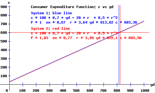
Consumers (Individuals).

The Consumer Expenditure Function.

c = c(yd, r)

c = c1 + c2*yd - c3*r + c4*r²

c1, c2, c3, c4 >= 0

c = 100 + 0.7*yd - 20*r + 0.5*r²

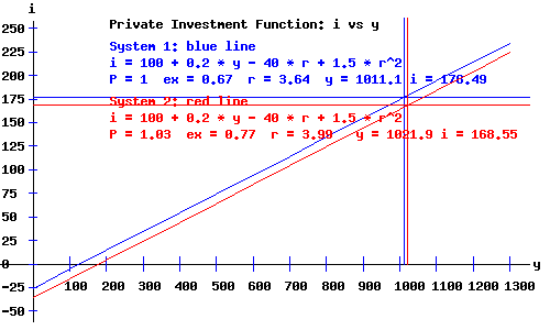
Producers (Firms).

The Private Firms' Investment Function.

i = i(y, r)

i = i1 + i2*y - i3*r + i4*r²

i1, i2, i3, i4 >= 0

i = 100 + 0.2*y - 40*r + 1.5*r²

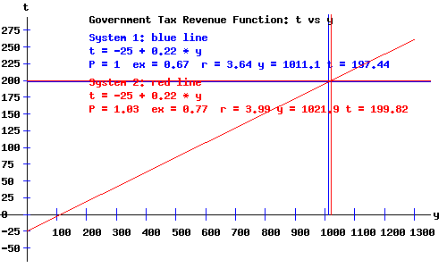
The Government.

Revenues and the Tax Function.

t = t(y)

t = -t1 + t2*y

t1, t2 >= 0

t = -25 + 0.22*y.

Disposable Income

Disposable national income, yd equals national income less taxes:

System 1:

yd = y - (-25 + 0.22*y) = 25 + 0.78*y = 25 + 0.78 * 1011.06 = 813.62.

System 2:

yd = y - (-25 + 0.22*y) = 25 + 0.78*y = 25 + 0.78 * 1021.92 = 822.1.

Government Expenditures.

In this basic macroeconomic model, I fixed government expenditures g = 210 billion dollars.

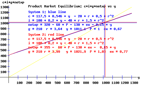
The Product (Commodity) Market Equilibrium.

The commodity markets equilibrate the demand and supply for exports and imports, consumer goods and services, investment goods, and goods and services purchased by the government. I aggregate the value of these products into one generic good.

I assume that the value of the supply of products produced (and hence national income) will adjust to meet the value of the demand for products —> aggregate supply, AS = aggregate demand, AD.

The product market equilibrium occurs at the level of national income where AD = AS, i.e., the level of income y where c + i + g + netxp = y. The diagram below depicts the equilibrium where c + i + g + netxp crosses the line (in yellow) with a 45 degree angle with the y-axis.

The c + i + g + netxp curve as a function of y and r is:

System 1:

c + i + g + netxp = 600.4 + 0.596*y - 60*r + 2*r²

System 2:

c + i + g + netxp = 620.6 + 0.596*y - 60*r + 2*r²

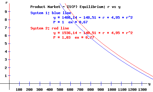
The IS(P) Curve.

With the price level (GDP deflator) and the exchange rate as part of the model through the net export function, the location of the equilibrium in the product market depends on the values of P and ex

The locus of interest rates and national incomes implicit for equilibrium in the commodity (product) market, an inverse relation between the rate of interest and national income, is called the IS(P) curve.

The IS(P) curve, y as a function of the rate of interest r, is:

System 1:

y = 1486.14 - 148.51 * r + 4.95 * r²

System 2:

y = 1536.14 - 148.51 * r + 4.95 * r²

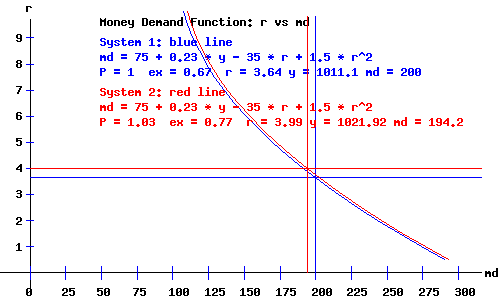
The Money Demand Function (Consumers and Producers).

md = md(y, r)

md = m1 + m2*y - m3*r + m4*r²

m1, m2, m3, m4 >= 0

md = 75 + 0.23*y - 35*r + 1.5*r²

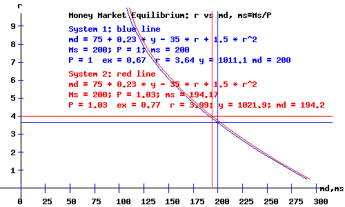
Money Supply.

I fixed the money supply ms = 200 billion dollars.

With the price level (GDP deflator) as part of the model, the real supply of money, ms, equals the nominal supply of money, Ms, divided by the price level, P.

System 1:

With a price level of P = 1, and a nominal money supply of Ms = 200, the real money supply is:

ms = Ms / P = 200.

System 2:

With a price level of P = 1.03, and a nominal money supply of Ms = 200, the real money supply is:

ms = Ms / P = 194.17.

The Money Market Equilibrium.

System 1:

With a price level of P = 1, a nominal money supply of Ms = 200, and national income of y = 1011.1, the equilibrium equation is:

200 = 307.54 - 35*r + 1.5*r²

with an equilibrium rate of interest r = 3.64.

System 2:

With a price level of P = 1.03, a nominal money supply of Ms = 200, and national income of y = 1021.9, the equilibrium equation is:

194.17 = 310.04 - 35*r + 1.5*r²

with an equilibrium rate of interest r = 3.99.

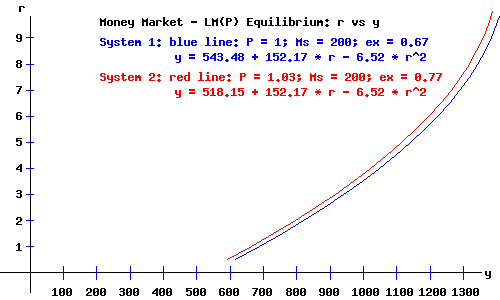
The LM(P) Curve.

y = (Ms/P - m1)/m2 + m3/m2 * r - m4/m2 * r²;

System 1:

For a price of P = 1, and nominal money supply Ms = 200:

The LM(P) curve, y as a function of the rate of interest r, is:

y = 543.48 + 152.17 * r - 6.52 * r²

System 2:

For a price of P = 1.03, and nominal money supply Ms = 200:

The LM(P) curve, y as a function of the rate of interest r, is:

y = 518.15 + 152.17 * r - 6.52 * r²

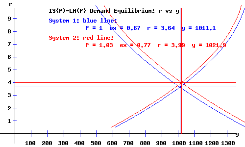
The IS(P)-LM(P) Demand Equilibrium.

The IS(P)-LM(P) economy is in equilibrium when national income, y, the rate of interest, r, the price level, P, and the exchange rate, ex, are at levels consistent with equilibrium in both the product and money markets.

Economy equilibrium occurs where the IS(P) curve and the LM(P) curve intersect.

As a review, I list the system of equations for the IS(P)-LM(P) model. Solving these equations simultaneously, I obtain the values of the endogenous macroeconomics variables of the model: the amount of output and national income, y, and the rate of interest, r.

For this basic model of the Canadian economy, the equilibrium obtains where:

System 1:

y = 1011.06,     r = 3.64 ,     P = 1 ,     ex = 0.67

System 2:

y = 1021.92,     r = 3.99 ,     P = 1.03 ,     ex = 0.77

The diagram below depicts the IS(P)-LM(P) economy demand equilibrium.

Economy Equilibrium Macroeconomic Variables and Aggregates