Employment, Price Level, and Output of Products.

The Keynesian IS-LM model focuses on the "demand side" of the economy - the relationship between national income and the aggregate demand for product (goods and services) by consumers, producers, and governments. The IS-LM model ignores the price level of goods and services, the level of employment, the wage rate of workers, and the amount of output of product. To include these macroeconomics aggregates in the model, I combine the labour market with the aggregate relationship between employment of workers and the level of output of product, providing the aggregate supply equation - a relationship between the price level and the level of output produced by firms. I also modify the equations that describe the money market of the basic IS-LM model to reflect the effect that changes in the price level have on the perceived "real supply" of money, yielding the aggregate demand equation - a relationship between the price level and the demand for output of firms.

The intersection of the aggregate demand and aggregate supply equations will yield the equilibrium level of output, the price level, the wage rate, and the level of employment, along with the rate of interest and the values of all the other macroeconomics variables obtained from the IS-LM model. This aggregate demand-aggregate supply (AD-AS) economics model tries to approximate the relationships among these key macroeconomics aggregates.

Below, I specify the functions (equations) that describe the aggregate activities of firms and workers in the production of goods and services: the production of output by firms from the factors of production, the private firms' demand for labour, and workers' supply of labour.

I set the values of the parameters of the macroeconomics functions to reflect the average values of the macroeconomics aggregates of the Canadian economy during the years of 1998 - 2003. (Statistics Canada: Gross domestic product, income-based;   Gross domestic product, expenditure-based. )   I express all aggregates in billions of dollars.

In setting the values of these parameters, I have been concerned with obtaining a system of equations that fit the data (reasonably). If you have better estimates for the values of these parameters, you can modify the model within limits on the web page: Comparative Statics Of The AD-AS Model.

The Aggregate Production Function.

The aggregate production function relates the amount of output produced in the economy to the amounts of inputs used, the amounts of labour, capital, and materials & supplies actively employed. Labour, capital, and materials & supplies are called the factors of production. Increasing the amount of any factor of production, while holding constant the other factors, will increase the amount of output. In this basic short-run AS-AD model, I consider the effect on output of varying the amount of labour employed, assuming materials & supplies vary in direct proportion to labour. Capital (more properly, capital services) are constant over the relevant time period of the model. The aggregate production function specifies the relation between labour inputs and the output of the firms in the economy. Since the contribution to output of one hour of labour employed depends on the type of job, and on the experience and education of the person employed, I assume I can convert the sum of all labour inputs into one generic labour input.

The productivity of labour is the average amount of output produced from one hour of generic labour employed. Labour productivity is a function of the stock of capital, the experience and education of the labour force (called human capital), and the technology available to firms to produce output by efficiently using capital services with labour and materials & supplies inputs.

I approximate an economy's aggregate production function:

ys = ys(N, K, M)

showing that the value of output, ys, depends on the inputs of hours of labour, N, services of capital, K, and materials and supplies, M.

I obtain a reasonable approximation using a function of the form:

ys = ys1 + ys2 * N - ys3 * N² - ys4 * N³

ys1, ys2, ys3, ys4 >= 0

where N is labour employed, expressed in billions of hours per year, and ys is the value of output produced in one year, expressed in billions of dollars.

For the Canadian economy, I use:

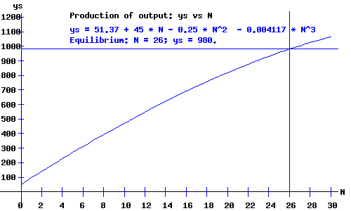
ys = 51.37 + 45 * N - 0.25 * N^2 - 0.004117 * N^3

The following diagram displays the graph of the aggregate production function relating output, ys, to labour, N, for a specific, but unspecified, stock of capital.

The shape and location of the aggregate production function depends on anything that influences the amount of output produced by firms in the economy. For example, an increase in labour productivity will tend to shift the aggregate production function upwards.

The Labour Market.

The Economy's Demand for Labour.

From microeconomics, I know that a profit maximizing firm's demand for labour depends on the marginal product of labour — the increase in output obtained from increasing the input of labour by one hour. The marginal product of labour function for a firm is the derivative of that firm's microeconomic production function (as a function of labour employed) with respect to labour input. Firms will tend to increase labour input until the increase in the value of output of the last hour of labour added just matches the increase in costs, as given by the wage rate per hour of labour input.

To maintain this relation between the aggregate production function and the aggregate demand for labour for the AD-AS model, I obtain the aggregate demand for labour function by differentiating the aggregate production function with respect to N.

Therefore, the aggregate labour demand function has the form:

wd = wd1 - wd2 * N - wd3 * N²

wd1 = ys2, wd2 = 2 * ys3, wd3 = 3 * ys4

From the aggregate production function above this is:

wd = 45 - 0.5 * N - 0.01235 * N^2

In situations with excess capital stock (some machinery and equipment sits idle), the demand for labour schedule might not be the derivative of the aggregate production function with respect to labour. If output is increased, idle capital could combine more efficiently (at lower cost) with added labour, than capital that is already being used. Technically, capital stock can be a variable factor of production, even in the short-run. However, this phenomenon can be modelled by adjusting the shape of the production function. In other words, the shape of the production function and the labour demand function depend on what I mean when I say capital stock is fixed in the short-run.

The Economy's Supply of Labour.

Economists usually derive the supply of labour as a function of the wage rate by examining the trade-off between work and leisure. Workers want to work more hours and additional people enter the work force as the wage rate increases. Eventually, when a worker's income reaches a threshold, a worker will want to increase leisure time.

In the long run, the real wage rate (adjusted for the rate of inflation in prices) determines the number of hours of labour supplied to firms.

As the number of people participating in the work force increases, the aggregate supply schedule will "shift" to the right as people offer more hours of work to firms at each wage rate.

I capture these features of the labour market in the following labour supply function:

ws = ws1 + ws2 * N + ws3 * N²

ws1, ws2, ws3 >= 0

For the Canadian economy, I use:

ws = 0 + 0.5 * N + 0.01575 * N^2

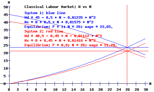
Classical Labour Market.

In the long run, firms and workers adjust their demand and supply in the labour market with reference to both the price level and the money wage rate.

labour demand: wd = Wd / P --> Wd = P * wd = P * (wd1 - wd2 * N - wd3 * N²)

labour supply: ws = Ws / P --> Ws = P * ws = P * (ws1 + ws2 * N + ws3 * N²)

where P is the price level (GDP deflator), and Wd and WS are the demand and supply money wage rates (wage rates in current dollars), respectively.

The intersection of the labour demand and labour supply schedules yields the equilibrium money wage rate and level of employment.

Both the labour demand and supply functions shift with the price level, P. The equilibrium money wage, W, and level of employment, N, for price levels of P = 1.0 and P = .90 are shown in the following diagram. Notice that in the model of the Classical Labour Market, the equilibrium level of employment remains constant, while the labour market's equilibrium money wage rate changes proportionally to the change in the price level.

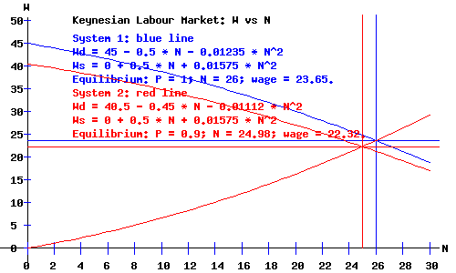
Keynesian Labour Market.

In the short run, employers and unions enter into binding labour contracts that specify workers' wage rates, while the prices of products, particularly consumer goods, are free to fluctuate. While labour contracts may include inflation adjustment clauses, the prices of outputs are relatively flexible, while wage rates (including minimum wage rates) are relatively fixed.

I capture this flexible money price for goods, fixed money wage for labour short-run dichotomy by letting the price level, P, shift the labour demand schedule, Wd but not the labour supply schedule, Ws.

labour demand: Wd = P * (wd1 - wd2 * N - wd3 * N²)

labour supply: Ws = ws1 + ws2 * N + ws3 * N²)

The intersection of the labour demand and labour supply schedules yields the equilibrium money wage rate and level of employment.

The equilibrium money wage rates, W, and levels of employment, N, for price levels of P = 1 and P = 0.9 are shown in the following diagram. Notice that in the model of the Keynesian Labour Market, the equilibrium level of employment and the equilibrium money wage rate change in response to a change in the price level. A reduction in the price level, P, reduces the money wage rate, W, and level of employment, N .

Aggregate Supply.

An economy's aggregate supply schedule describes the relationship between the price level (GDP deflator) and the amount of output produced by enterprises. In the long run, if the prices of products and prices of factor inputs remain in the same proportion, the aggregate supply schedule will be vertical. In the short run, if the prices of products can increase or decrease relative to the prices of factor inputs, the aggregate supply schedule will have a positive slope.

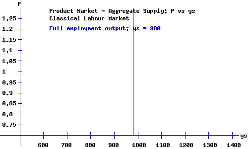
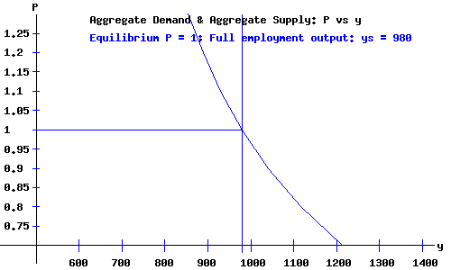
Classical Aggregate Supply.

The location of the vertical Classical aggregate supply schedule depends on the economy's aggregate production function and on the labour supply schedule. The level of employment and amount of output are the "full employment" levels for the economy.

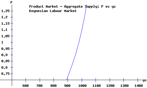
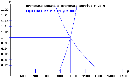
Keynesian Aggregate Supply.

The location (and shape) of the positively-sloped Keynesian aggregate supply schedule depends on the economy's aggregate production function, on the aggregate labour supply schedule, and on the extent to which a change in the price level shifts the aggregate demand for labour schedule relative to the shift in the aggregate supply of labour schedule. I assume that the price level shifts the labour demand schedule proportionally, while the aggregate supply schedule remains "stationary."

The Price Level and the Money Market.

Click for a detailed description of the money market without the complication of the price level. With the price level (GDP deflator) as part of the model, the real supply of money, ms, equals the nominal supply of money, Ms, divided by the price level, P.                                

For equilibrium to obtain in the money market at a given level of national income, y, the rate of interest, r, adjusts until the real supply of money equals the demand for money.

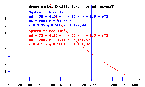
Using the coefficients from the demand for money and supply of money functions, the equilibrium equation is:

Ms / P = ms = md = m1 + m2*y - m3*r + m4*r²

              = 75 + 0.23*y - 35*r + 1.5*r²

With a price level of P = 1, a nominal money supply of Ms = 200, and national income of y = 980, the equilibrium equation is:

200 = 300.4 - 35*r + 1.5*r²

with an equilibrium rate of interest r = 3.35.

With a price level of P = 1.1, a nominal money supply of Ms = 200, and national income of y = 980, the equilibrium equation is:

181.82 = 300.4 - 35*r + 1.5*r²

with an equilibrium rate of interest r = 4.11.

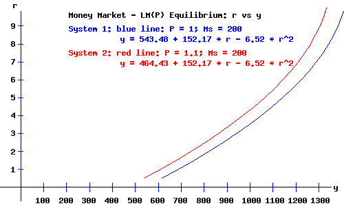
The LM(P) Curve.

Recall that the LM curve is the locus of interest rates and national incomes implicit for equilibrium in the money market, a direct relation between the rate of interest and national income. I relabel the LM curve as LM(P) to indicate that it also depends on the price level. The equation of the LM(P) curve, y as a function of the rate of interest, r, and the price level, P, is:

y = (Ms/P - m1)/m2 + m3/m2 * r - m4/m2 * r²;

where the coefficients come from the demand for money and supply of money functions.

For a price of p = 1, and nominal money supply Ms = 200:

y = 543.48 + 152.17 * r - 6.52 * r².

y = 464.43 + 152.17 * r - 6.52 * r².

The LM(P) curve shifts to the left as the price level increases.

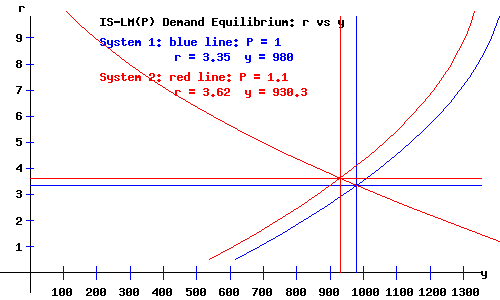
The IS-LM(P) Demand Equilibrium.

Recall that the IS curve is the locus of interest rates and national incomes implicit for equilibrium in the product (commodity) market, an inverse relation between the rate of interest and national income. I assume that the IS curve does not shift with changes in the price level. (Click to see a detailed description of the IS curve.)

The basic IS-LM(P) economy model is in equilibrium when national income, y, and the rate of interest, r, and the price level, P, are at levels consistent with equilibrium in both the product and money markets.

The economy's demand equilibrium occurs where the IS curve and the LM(P) curve intersect.

When P = 1, the equilibrium demand equilibrium occurs with a demand for product of y = 980, at a rate of interest r = 3.35.

When P = 1.1, the equilibrium demand equilibrium occurs with a demand for product of y = 930.3, at a rate of interest r = 3.62.

The diagram below shows the economy's IS-LM(P) demand equilibrium.   A higher price level implies an economy equilibrium with a lower aggregate demand for products (commodities).

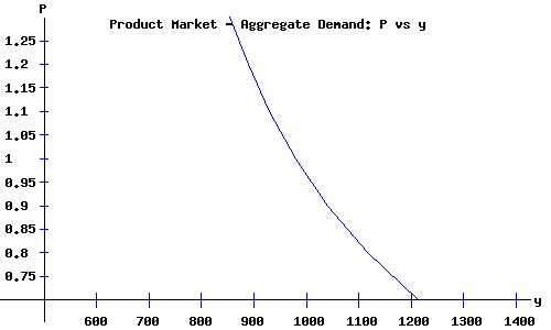
Aggregate Demand.

The aggregate demand curve is the locus of price levels and national demand for product ( = national income) implicit for equilibrium in the product (commodity) market. A decrease in the price level yields a greater demand for product. The aggregate demand curve is negatively sloped. Its location and shape depends on the demand for consumer goods, the demand for investment goods, the income tax schedule, government demand for goods (government expenditures), the demand for money, and the nominal supply of money.

Economy Equilibrium: Aggregate Demand and Supply.

As a review, I list the system of equations for the AD-AS model. Solving these equations simultaneously, I obtain the values of the endogenous macroeconomics variables of the model: the price level, P; the amount of output and national income, y; the rate of interest, r; the level of employment, N; and the wage rate, W. (Recall that the IS-LM(P) equilibrium obtains national income equal to aggregate demand for products.) On this web page, the Classical and the Keynesian models yield the same values for the endogenous variables P, y, r, N, and W, and the other derived macroeconomics aggregates. On the AD-AS comparative statics web page, you have the opportunity to set the values of the parameters of the model, permitting the Classical and Keynesian models to yield differing results.

Classical Economy Equilibrium.

Keynesian Economy Equilibrium.

Economy Equilibrium Macroeconomic Variables and Aggregates