Egwald Mathematics: Nonlinear Dynamics:

One Dimensional Dynamics and Bifurcations

by

Elmer G. Wiens

Egwald's popular web pages are provided without cost to users.
Please show your support by joining Egwald Web Services as a Facebook Fan:
Follow Elmer Wiens on Twitter:

one dimensional dynamics | introduction | difference equation | fixed points | stability analysis | higher order maps
bifurcations | saddle-node bifurcation | saddle-node example | flip bifurcation | second order map | saddle-node conditions
flip bifurcation conditions | flip bifurcation example | transcritical bifurcation | transcritical example | transcritical conditions
pitchfork bifurcation | pitchfork example | pitchfork conditions | references

One Dimensional Dynamics: Discrete Time Models.

Introduction

Continuous time, dynamic process are modelled with differential equations.  Discrete time, dynamic processes are modelled with difference equations. Consider a dynamic process where the rate of change of a variable from one time period to the next is proportional to magnitude of the variable.

Writing x_t as the magnitude of the variable at time t, the dynamic process modelled as a difference equation is:

x_t+1 = x_t + k * x_t = (1 + k) * x_t,   x₀ = x0,         (1)

where the constant k is the rate of change, and x0 is the magnitude of the variable at the start, time t = 0.

The solution to this difference equation is the discrete function of time, x(t, x0), for t an integer:

x(t, x0) = {x₀, x₁, x₂,  . . .   x_n,   ...   },

providing the time profile of the magnitude of x with an initial value of x0.

The sequence of numbers, {x₀, x₁, x₂,  . . .   x_n,   ...   }, is called an orbit.

One can solve the difference equation, (1), by induction:

Writing λ = (1 + k), the difference equation (2) and its solution (3) are:

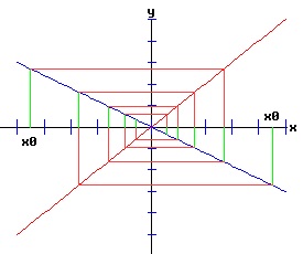
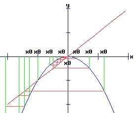
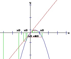
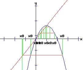
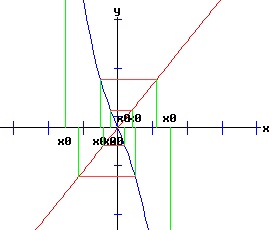
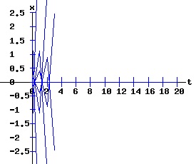
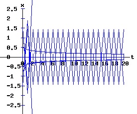
The solution x(t, x0) = λ^t * x0 suggests that the variable x will grow or decay exponentially from its starting population, x0, at a rate depending on the value of the parameter λ. If x0 > 0, and if λ > 1 (k > 0), the variable x increases in value; but if x0 > 0, and if λ < 1 (k < 0), the variable x decreases in value. Conversely, if x0 < 0, and if λ > 1 (k > 0), the variable x decreases in value; but if x0 < 0, and if λ < 1 (k < 0), the variable x increases in value.

One can see the evolution of these solutions in the following staircase diagrams:

In the first set of diagrams, the green lines touch the x-axis at x0, x₁, x₂, x₃, etc. In both diagrams |x0| > |x₁| > |x₂| > |x₃| > ... |x_t| > ... → 0, but in the second diagram the x_t alternate in sign.

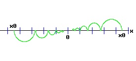
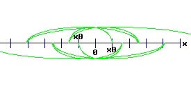
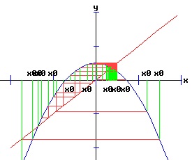
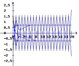
The second set of diagrams above display the phase portraits of the difference equation, showing the movement of x_t along the x-axis for t = 0, 1, 2, ... etc. This sequence converges to x^* = 0 for any initial x0. The basin of attraction of x^* = 0 is said to be the interval (-∞, ∞), since any initial x0 converges to 0.

In the first set of diagrams below, the green lines touch the x-axis at x0, x₁, x₂, x₃, etc. In both diagrams 0 < |x0| < |x₁| < |x₂| < |x₃| < ... < |x_t| < ... → ∞ , but in the second diagram the x_t alternate in sign.

The second set of diagrams above are the phase portraits of the difference equation, displaying the movement of x_t along the x-axis for t = 0, 1, 2, ... etc. This sequence diverges for any initial x0 except x0 = 0. Thus, the basin of attraction of x^* = 0 is the single point 0.

One Dimensional Difference Equations

The general form of a one dimensional difference equation with a parameter r is:

x_t+1 = f(x_t, r),   x₀ = x0.         (4)

where f is a function of x and r.

Difference equations are also called maps, recursion relations, or iterated maps.

Fixed Points

For a specific value of the parameter r = r1 it is sometimes convenient to write:

f(x, r1) = f(x).         (5)

f(x^*) = x^*.         (6)

Stability Analysis

One can analyze the local stability of the difference equation (4) about a fixed point by examining the first derivative of the function f with respect to x evaluated at x^* (the partial derivative of f with respect to x evaluated at x^*):

λ = f'(x^*) = f_x(x^*, r).         (7)

where λ is called the multiplier or eigenvalue, determining the stability of (4) at x^*.

The discrete time, dynamic process determined by the function f is stable at x^* if:

|λ| = f'(x^*) < 1,

and super-stable if:

|λ| = f'(x^*) = 0;

the process is unstable at x^* if:

|λ| = f'(x^*) > 1.

If f is stable at x^*, x^* is called an attractor.   If f is unstable at x^*, x^* is called a repeller.

If |λ| ≠ 1, x^* is called a hyperbolic fixed point.

The stability of the process must be examined for each situation if:

|λ| = f'(x^*) = 1.

If |λ| = 1, x^* is called a non-hyperbolic fixed point.

Higher Order Maps

The second order map, f², for the function f in (4) is given by:

x_t+2  =  f(x_t+1, r)  =  f (f(x_t, r), r )  =   f²(x_t, r)

The third order map, f³, is given by:

x_t+3  = f( f (f(x_t, r), r), r)  =   f³(x_t, r).

Repeat this sequence for the 4th, 5th, etc. order maps.

One Dimensional Bifurcations.

A dictionary definition of bifurcation states: Division into two branches; the point of division; the branches or one of them.

A nonlinear process experiences a qualitative change in its dynamics when the nature of its fixed points change. When a change in a parameter results in a qualitative change in the dynamics of a nonlinear process, the process is said to have gone through a bifurcation.

A one dimensional, discrete time, nonlinear dynamic process is modelled by the function f of two variables, x and r, where f is nonlinear in x, and r is a parameter. The difference equation governing the dynamics of the process is:

x_t+1 = f(x_t, r),   x₀ = x0.         (8)

Bifurcations are classified by the way in which the fixed points of the function f change their number, location, form, and stability. It is convenient to consider normal forms for the different types of bifurcations, and the conditions under which the dynamic process described by equation (8) will experience a specific type of bifurcation.

Discrete time dynamical systems may experience saddle-node, transcritical, and pitchfork bifurcations that are similar to their continuous time counterparts. The flip bifurcation is unique to discrete time dynamical processes.

A bifurcation can only occur at a non-hyperbolic fixed point.

Saddle-Node Bifurcation

The normal form of a discrete time process with a saddle-node bifurcation with parameter r is:

f(x, r) = a * r + b * x²,   a ≠ 0,   b ≠ 0.         (9)

Fixed points of equation (9) satisfy:

f(x, r) = a * r + b * x² = x.         (10)

Fixed points are the roots of the quadratic equation:

b * x² - x + a * r = 0.           (11)

For a specific value of the parameter r, the roots of equation (11) are:

x₁ = (1 + sqrt(1 - 4 * b * a * r)) / (2 * b) ,         (12)

x₂ = (1 - sqrt(1 - 4 * b * a * r)) / (2 * b).         (13)

Linearized Stability:

The stability of f at a fixed point, x_i, is determined by the partial derivative of f with respect to x evaluated at the fixed point (ie the multiplier or eigenvalue of f):

λ_i = f_x(x_i, r) = 2 * b * x_i.         (14)

Substituting (12) and (13) into (14) yields:

λ₁ = 1 + sqrt(1 - 4 * b * a * r),

λ₂ = 1 - sqrt(1 - 4 * b * a * r)

If the parameter r takes on the critical value:

r_c = 1 / (4 * b * a),

the repeated fixed point is:

x_1,2 = 1 / (2 * b),

with multiplier:

λ_1,2 = 1 .

Consequently, ( x_1,2, r_c) = (1 / (2 * b),   1 / (4 * b * a) ) is a non-hyperbolic fixed point. In fact, it is a saddle-node bifurcation point.

Furthermore,

λ₂ = 1 - sqrt(1 - 4 * b * a * r)  =  -1,   if

r_c = -3 / (4 * b * a).

The fixed points are:

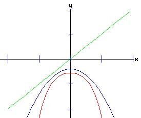
x₁ = (1 + sqrt(1 + 3)) / (2 * b) = 3 / (2 * b),

x₂ = (1 - sqrt(1 + 3)) / (2 * b) = -1 / (2 * b).

Consequently, ( x₂, r_c) = (-1 / (2 * b),   -3 / (4 * b * a) ) is also a non-hyperbolic fixed point. In fact, it is a flip bifurcation point.

Saddle-Node Bifurcation: a = 1, b = -1;   ( x_1,2,  r_c) = (- 1 / 2,  - 1 / 4 )

The prototype function f is:

f(x, r) = r - x²,         (15)

whose fixed points satisfy:

r - x₂  =  x.

The fixed points and multipliers are:

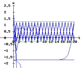
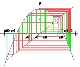
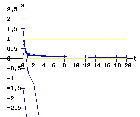
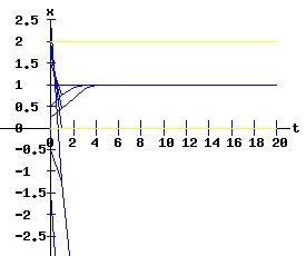
x₁ = (-1 - sqrt(1 + 4 * r)) / 2,   λ₁ = 1 + sqrt(1 + 4 * r)

x₂ = (-1 + sqrt(1 + 4 * r)) / 2,   λ₂ = 1 - sqrt(1 + 4 * r)

The values of x₁ and x₂ are complex when r < -1 / 4, and the dynamic process has no fixed points here.

When r = -1 / 4, x₁ = x₂ = -1 / 2, and λ₁ = λ₂ = 1. The basin of attraction of the fixed point -1 / 2 is the closed interval [x₁, -x₁] = [-1/2,  1/2], since trajectories starting at x0 in this interval converge to -1 / 2.

When -1 / 4 < r < 3 / 4, λ₁ > 1 and -1 < λ₂ < 1. Consequently, x₁is a repeller (unstable), and x₂ is an attractor (stable). The basin of attraction for the attractor x₂ is [x₁, -x₁].

The following diagrams display the phase diagrams and solution trajectories of x(t,  x0) for the discrete time, nonlinear dynamic process.

The yellow lines delimit the basin of attraction of the stable fixed point given by the closed interval [x₁, -x₁].

x_t+1 = r - x_t²,   x₀ = x0.

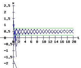
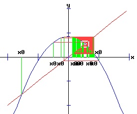
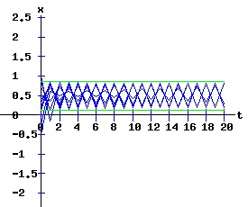
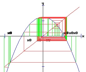
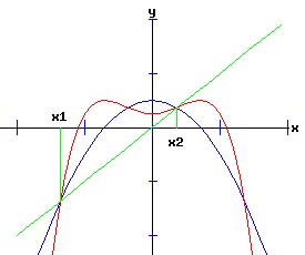
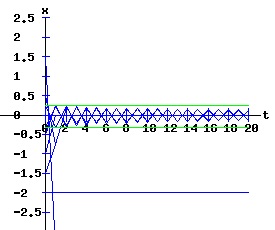
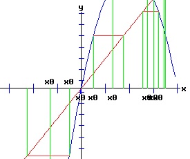
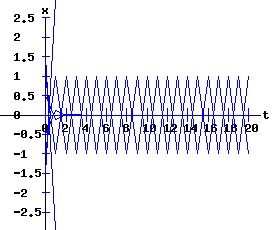
Flip Bifurcation: a = 1, b = -1;   ( x₂,  r_c) = ( 1 / 2,  3 / 4 )

As r increases past 3 /4, the fixed point x₂ loses its stability, flipping from an attractor to a repeller. The following diagrams display the phase diagrams and solution trajectories of x(t,  x0) for the discrete time, nonlinear dynamic process. The green lines delimit the minimal trapping region. If x_t0 lands in the trapping region for some value of t₀, x_t remains in the trapping region for t > t₀. This trapping region is the closed interval [f(0, r), f(f(0, r), r)], where f²(x, r) = f(f(x, r), r) is the second order map discussed below.

x_t+1 = r - x_t²,   x₀ = x0.

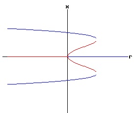
The Second Order Map of f

The second order map of f as stated in (15) is the a fourth-order polynomial in x:

x_t+2  =  f(x_t+1, r)  =  f (f(x_t, r), r ) = r - (r - x_t²)² = r - r² + 2 * r * x_t² - x_t⁴.         (16)

Denote this mapping by f²:

f²(x, r) = r - r² + 2 * r * x² - x⁴,         (17)

whose partial derivative with respect to x is:

f_x²(x, r) = 4 * r * x - 4 * x³.         (18)

Fixed points of (17) satisfy:

f²(x, r) = r - r² + 2 * r * x² - x⁴ = x.         (19)

The fixed points of f² are:

x₁ = (-1 - sqrt(1 + 4 * r)) / 2,

x₂ = (-1 + sqrt(1 + 4 * r)) / 2,

x₃ = (1 + sqrt(-3 + 4 * r)) / 2,

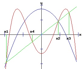
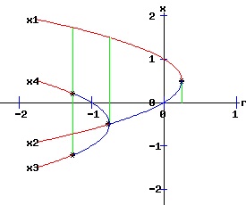
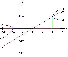
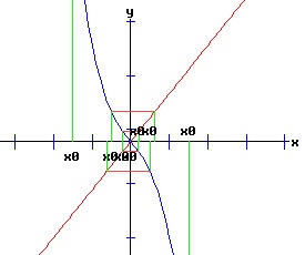
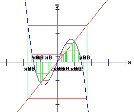
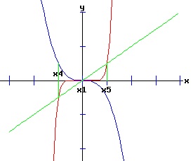
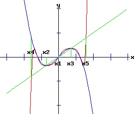
x₄ = (1 - sqrt(-3 + 4 * r)) / 2

The first two fixed points of f²are also fixed points of f.   The stability of the fixed points of f² provide information on the bifurcation points and solution trajectories of f.

The following graphs display the phase diagrams of f in blue and f² in red.

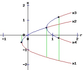
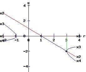
At (x, r) = (-1 / 2, -1 / 4), f and f² have a slope of 1, and f saddle-node bifurcates into two fixed points, one unstable and the other stable. At (x, r) = (1 / 2, 3 / 4), f has a slope of -1, while f² has a slope of 1. At this flip bifurcation, the stability of f flips from stable to unstable. Meanwhile, the fixed point of f² splits into three fixed points, bracketing the unstable fixed point that it shares with f with two stable fixed points, x₃ and x₄.   At r = 1.25, the fixed points x₃ and x₄ of f² flip from stable to unstable.

The following bifurcation diagram summarizes the behaviour of the fixed points. It shows the fixed points as a function of the parameter r. The blue curves represent the stable fixed points, while the red curves represent the unstable fixed points. The bifurcation points are marked with an asterisk, *.

This discrete time, saddle-node bifurcation diagram is similar to the continuous time, type two saddle-node bifurcation diagram.

The normal form of a discrete time process with a saddle-node bifurcation is:

x_t+1 = f(x_t,  r) = a * r + b * x_t²,   x₀ = x0,   a ≠ 0,   b ≠ 0.         (20)

Saddle-Node Conditions

The discrete time, dynamic process described by equation (20) undergoes a saddle-node bifurcation at (x^*,  r_c) if:

The bifurcation diagrams for the four types of saddle-node bifurcations are displayed below. The fixed points of f are x₁ and x₂, while the fixed points of f² are x₁, x₂, x₃, and x₄. These fixed points are graphed as functions of the parameter, r. The discrete time, dynamic process undergoes a flip bifurcation when the stability of the fixed point, x₂, flips. At this critical value of r, the stable fixed points x₃ and x₄ of f² emerge and bracket x₂.

The blue curves represent the stable fixed points, while the red curves represent the unstable fixed points. The bifurcation points are marked with an asterisk, *.

Flip Bifurcation Conditions (Lorenz 111)

Consider the discrete time, dynamic process given by:

x_t+1 = f(x_t,  r),   x₀ = x0.         (22)

If the fixed point x = x^* and parameter value r = r_c satisfy:

then, depending on the signs of the expressions in (F3) and F4),

1. the fixed point x^* is stable (unstable) for r < r_c (r > r_c), and

2. the fixed point x^* becomes unstable (stable) for r > r_c (r < r_c); moreover, a branch of stable (unstable) fixed points of order 2 (ie fixed points of f²) emerges which bracket x^*.

Supercritical Flip Bifurcation (Period Doubling Bifurcation)

If c < 0 in expression F4, the emerging fixed points of f² are stable and bracket an unstable fixed of f. The trajectory x_t switches between the two attracting fixed points of f².

Subcritical Flip Bifurcation

If c > 0 in expression F4, the emerging fixed points of f² are unstable and bracket a stable fixed of f.    See the supercritical pitchfork example for an example of a subcritical flip bifurcation.

Supercritical (Period Doubling) Flip Bifurcation Example

The discrete time, dynamic process:

x_t+1 = f(x_t, r) = r - x_t²,   x₀ = x0.

with:

undergoes a flip bifurcation at (x₂, rc) = (1 / 2, 3 / 4) as r increases, where the stability of the fixed point x₂ of f flips from stable to unstable, and two stable fixed points x₃ and x₄ of f² emerge bracketing x₂.

Checking the flip bifurcation conditions:

The supercritical flip bifurcation conditions are satisfied with c < 0.

Transcritical Bifurcation

The normal form of a discrete time process with a transcritical bifurcation with parameter r is:

x_t+1 = f(x_t,  r) = a * r * x_t + b * x_t²,   x₀ = x0,   a ≠ 0,   b ≠ 0.         (24)

The fixed points of f satisfy:

f(x, r) = a * r * x + b * x² = x.         (25)

For a specific value of the parameter r, the roots of equation (25) are:

x₁ = 0 ,         (26)

x₂ = (1 - a * r) / b.         (27)

Linearized Stability:

The stability of f at a fixed point, x_i, is determined by the partial derivative of f with respect to x

f_x(x, r) = a * r + 2 * b * x,         (28)

evaluated at the fixed point (ie the multiplier or eigenvalue of f):

λ_i = f_x(x_i, r) = a * r + 2 * b * x_i.         (29)

Substituting (26) and (27) into (29) yields:

λ₁ = a * r,

λ₂ = - a * r + 2

If the parameter r takes on the critical value:

r_c = 1 / a,

the repeated fixed point is:

x_1,2 = 0,

with multiplier:

λ_1,2 = 1 .

Consequently, ( x_1,2, r_c) = (0,   1 / a) is a non-hyperbolic fixed point. In fact, it is a transcritical bifurcation.

Furthermore,

λ₁ = a * r   =   -1,   if

r_c = -1 / a.

The fixed points are:

x₁ = 0,

x₂ = 2 / b.

Consequently, ( x₁, r_c) = (0,   -1 / a) is also a non-hyperbolic fixed point. In fact, it is a flip bifurcation.

Moreover,

λ₂ = - a * r + 2   =   -1,   if

r_c = 3 / a.

The fixed points are:

x₁ = 0,

x₂ = -2 / b.

Consequently, ( x₂, r_c) = (-2 / b,   3 / a) is also a non-hyperbolic fixed point. In fact, it is a flip bifurcation.

Transcritical Bifurcation: a = 1, b = -1;   ( x_1,2,  r_c) = (0,   1 )

The prototype function f is:

f(x, r) = r * x - x²,         (30)

whose fixed points satisfy:

r * x - x₂  =  x.

The fixed points and multipliers are:

x₁ = 0,   λ₁ = r

x₂ = -(1 - r),   λ₂ = - r + 2

The values of x₁ and x₂ are real for all r.

For -1 <= r <= 1, x₁ is an attractor, while x₂ is a repeller. Conversely, for 1 < r <= 3, x₁ is a repeller, while x₂ is an attractor.

When r < 1, x₁ and x₂ are repellers (unstable fixed points). Similarly, when r > 3, x₁ and x₂ are repellers.

The following diagrams display the phase diagrams and solution trajectories of x(t,  x0) for the discrete time, nonlinear dynamic process:

x_t+1 = r * x_t - x_t²,   x₀ = x0.

The yellow linesdelimit the basin of attraction of the stable fixed point. The green lines delimit the minimal trapping region.

The Second Order Map of f

The second order map of f as stated in (30) is the a fourth-order polynomial in x:

x_t+2  =  f(x_t+1, r)  =  f (f(x_t, r), r ) = r * (r - x_t²) - (r - x_t²)² = -x_t⁴ + 2 * r * x_t³ + (-r-r²) * x_t² + r² * x_t.         (31)

Denote this mapping by f²:

f²(x, r) = r² * x + (-r - r²) * x² + 2 * r * x³ - x⁴,         (32)

whose partial derivative with respect to x is:

f_x²(x, r) = r² + 2 * (-r - r²) * x + 6 * r * x² - 4 * x³.         (33)

Fixed points of (32) satisfy:

f²(x, r) = r² * x + (-r - r²) * x² + 2 * r * x³ - x⁴ = x.         (34)

The fixed points of f² are:

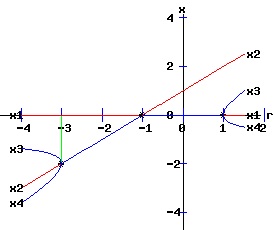
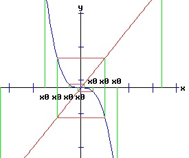
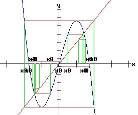
The first two fixed points of f²are also fixed points of f.   The stability of the fixed points of f² provide information on the bifurcation points and solution trajectories of f.

The following graphs display the phase diagrams of f in blue and f² in red.

At (x, r) = (0,  1), f and f² have slopes of 1 and 1, respectively. Here f transcritical bifurcates into two fixed points x₁ and x₂. For -1 < r < 1, x₁ is stable and x₂ is unstable. At (x, r) = (0, -1), f and f₂ have slopes of -1 and 1, respectively. At this flip bifurcation, the stability of x₁ flips from stable to unstable for r < -1. Meanwhile, the fixed point x₁ of f² splits into three fixed points, bracketing the unstable fixed point x₁ it shares with f with two stable fixed points, x₃ and x₄.   For 1 < r < 3, x₁ is unstable and x₂ is stable. At (x, r) = (x₂, 3), f and f₂ have slopes of -1 and 1, respectively. At this flip bifurcation, the stability of x₂ flips from stable to unstable for r > 3. Meanwhile, the fixed point x₂ of f² splits into three fixed points, bracketing the unstable fixed point x₂ it shares with f with two stable fixed points, x₃ and x₄.

The normal form of a discrete time process with a transcritical bifurcation is:

x_t+1 = f(x_t,  r) = a * r * x_t + b * x_t²,   x₀ = x0,   a ≠ 0,   b ≠ 0.         (35)

Transcritical Conditions

The bifurcation diagrams for the four types of transcritical bifurcations are displayed below. The fixed points of f are x₁ and x₂, while the fixed points of f² are x₁, x₂, x₃, and x₄. These fixed points are graphed as functions of the parameter, r. The discrete time, dynamic process undergoes supercritical flip bifurcations when the stability of the fixed points, x₁ and x₂, flip. At these critical values of r, the stable fixed points x₃ and x₄ of f² emerge and bracket x₁ or x₂.

The blue curves represent the stable fixed points, while the red curves represent the unstable fixed points. The bifurcation points are marked with an asterisk, *.

PitchFork Bifurcation

The normal form of a discrete time process with a pitchfork bifurcation with parameter r is:

x_t+1 = f(x_t,  r) = a * r * x_t + b * x_t³,   x₀ = x0,   a ≠ 0,   b ≠ 0.         (37)

Supercritical Pitchfork Bifurcation

In the normal form of a supercritical pitchfork bifurcation, the coefficient, b, in equation (37) is negative. Consequently, the cubic term stabilizes the dynamic process by pulling the trajectory of x(t) back toward x = 0.

Subcritical Pitchfork Bifurcation

In the normal form of a subcritical pitchfork bifurcation, the coefficient, b, in equation (37) is positive. Consequently, the cubic term destabilizes the dynamic process by driving the trajectory of x(t) toward infinity.

The fixed points of f satisfy:

f(x, r) = a * r * x + b * x³ = x.         (38)

For a specific value of the parameter r, the roots of equation (38) are:

x₁ = 0 ,         (39)

x₂ = sqrt(-b * (a * r - 1)) / b.         (40)

x₃ = -sqrt(-b * (a * r - 1)) / b.         (41)

The fixed points x₁ and x₂ are real if:

-b * (a * r - 1) > 0.         (42)

Linearized Stability:

The stability of f at a fixed point, x_i, is determined by the partial derivative of f with respect to x

f_x(x, r) = a * r + 3 * b * x²,         (43)

evaluated at the fixed point (ie the multiplier or eigenvalue of f):

λ_i = f_x(x_i, r) = a * r + 2 * b * x_i².         (44)

Substituting (39), (40), and (41) into (44) yields:

λ₁ = a * r,

λ₂ = -2 * a * r + 3

λ₃ = -2 * a * r + 3

If the parameter r takes on the critical value:

r_c = 1 / a,

the triple fixed point is:

x_1,2,3 = 0,

with multiplier:

λ_1,2,3 = 1 .

Consequently, ( x_1,2,3, r_c) = (0,   1 / a) is a non-hyperbolic fixed point. In fact, it is a pitchfork bifurcation.

Furthermore,

λ₁ = a * r   =   -1,   if

r_c = -1 / a,

with corresponding fixed point:

x₁ = 0.

With r = - 1 / a, the fixed points x₂ and x₃ are real if b > 0, with

x₂ = sqrt(2 * b) / b,

x₃ = -sqrt(2 * b) / b.

Moreover,

λ_2,3 = - 2 * a * r + 3   =   -1,   if

r_c = 2 / a.

With r = 2 / a, the fixed points x₂ and x₃ are real if b < 0, with

x₁ = 0,

x₂ = sqrt(- b) / b,

x₃ = -sqrt(- b) / b.

Supercritical PitchFork Bifurcation: a = 1, b = -1;   ( x_1,2,3,  r_c) = (0,   1 )

The prototype function f is:

f(x, r) = r * x - x³,         (45)

whose fixed points satisfy:

r * x - x₃  =  x.

The fixed points and multipliers are:

x₁ = 0,   λ₁ = r

x₂ = -sqrt(r - 1),   λ₂ = - 2 * r + 3

x₃ = sqrt(r - 1),   λ₂ = - 2 * r + 3

The values of x₂ and x₃ are real for all r >= 1.

For r < -1, x₁ is a repeller. At r = -1, x₁ flips to attractor. For -1 < r < 1, x₁ is an attractor. At r = 1, x₁ flips to repeller. For 1 < r <= 2, x₂ and x₃ are attractors. At r = 2, x₂ and x₃ flip to repellers for r > 2.

The following diagrams display the phase diagrams and solution trajectories of x(t,  x0) for the discrete time, nonlinear dynamic process:

x_t+1 = r * x_t - x_t³,   x₀ = x0.

The Second Order Map of f

The second order map of f as stated in (45) is the a ninth-order polynomial in x:

x_t+2  =  f(x_t+1, r)  =  f (f(x_t, r), r ) = r * (r - x_t³) - (r - x_t³)³ = x_t⁹ - 3 * r * x_t⁷ + 3 * r² * x_t⁵ + (-r - r³) * x_t³ + r² * x_t.         (46)

Denote this mapping by f²:

f²(x, r) = r² * x + (-r - r³) * x³ + 3 * r² * x⁵ - 3 * r * x⁷ + x⁹,         (47)

whose partial derivative with respect to x is:

f_x²(x, r) = r² + 3 * (-r - r³) * x² + 15 * r² * x⁴ - 21 * r * x⁶ + 9*x⁸.         (48)

Fixed points of (47) satisfy:

f²(x, r) = r² * x + (-r - r³) * x³ + 3 * r² * x⁵ - 3 * r * x⁷ + x⁹ = x.         (49)

These fixed points of f² are:

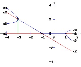
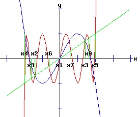
The first three fixed points of f²are also fixed points of f. When r >= 1, x₂ and x₃ are real numbers. When r >= -1, x₄ and x₅ are real numbers. When r >= 2, x₆, x₇, x₈, and x₉ emerge as real numbers.

The following graphs display the phase diagrams of f in blue and f² in red.

At (x, r) = (0,  1), f and f² each have a slope of 1; f pitchfork bifurcates with two new fixed points x₂ and x₃ emerging as r increases. At (x, r) = (0, -1), f and f₂ have slopes of -1 and 1, respectively. At this flip bifurcation, the stability of x₁ flips from unstable to stable as r increases. Meanwhile, the fixed point x₁ of f² splits into three fixed points, bracketing the stable fixed point x₁ it shares with f with two unstable fixed points, x₄ and x₅. For -1 < r < 1, x₁ is stable and x₄ and x₅ are unstable.   For 1 < r < 2, x₁ is unstable, while x₂ and x₃ are stable. At r = 2, f and f₂evaluated at x₂ and x₃ have slopes of -1 and 1, respectively. At this flip bifurcation, the stabilities of x₂ and x₃ flip from stable to unstable for r > 3. Meanwhile, the fixed points x₂ and x₃ of f² each split into three fixed points, bracketing the unstable fixed point shared with f with stable fixed points, x₆ and x₈ around x₂, x₇ and x₉ around x₃.

The normal form of a discrete time process with a pitchfork bifurcation is:

x_t+1 = f(x_t,  r) = a * r * x_t + b * x_t³,   x₀ = x0,   a ≠ 0,   b ≠ 0.         (35)

Note that f is an odd function since:

f(-x, r) = -f(x, r),

and therefore function f does not have a transcritical bifurcation since:

f_x,x(0, r) = 0.

Pitchfork Conditions

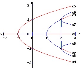
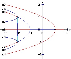
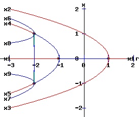
Bifurcation Diagrams

The bifurcation diagrams for the two types of supercritical and two types of subcritical pitchfork bifurcations are displayed below. The fixed points of f are x₁, x₂, and x₃, whereas the fixed points of f² are x₁, x₂, x₃, x₄, x₅, x₆, x₇, x₈, and x₉. These fixed points are graphed as functions of the parameter, r.

Supercritical Pitchfork Bifurcation Diagrams (b < 0)

The discrete time, dynamic process undergoes a pitchfork bifurcation at r = 1 / a where x₁ bifurcates into x₁, x₂, and x₃. A subcritical flip bifurcation occurs at r = -1 / a where the stability of the fixed point x₁ flips, and the unstable fixed points x₄ and x₅ of f² emerge bracketing the stable fixed point x₁ of f. Supercritical flip bifurcations occur at r = 2 /a where the stabilities of x₂ and x₃ flip from stable to unstable. Concurrently, the stable fixed points x₆ and x₈ of f² emerge bracketing x₂, and the stable fixed points x₇ and x₉ of f² emerge bracketing x₃.

The blue curves represent the stable fixed points, whereas the red curves represent the unstable fixed points. A bifurcation point is marked with an asterisk, *.

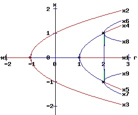
Subcritical Pitchfork Bifurcation Diagrams (b > 0)

The discrete time, dynamic process undergoes a pitchfork bifurcation at r = 1 / a where x₁ bifurcates into x₁, x₂, and x₃. A supercritical flip bifurcation occurs at the critical value of r = -1 / a where the stability of the fixed point x₁ flips. Concurrently, fixed points of f² emerge bracketing x₁ with x₄ and x₅. At r = -2 / a, the fixed point x₄ of f² bifurcates into x₄, x₆ and x₈; meanwhile the fixed point x₅ of f₂ bifurcates into x₅, x₇ and x₉.

The blue curves represent the stable fixed points, whereas the red curves represent the unstable fixed points. A bifurcation point is marked with an asterisk, *.

References.

• Burden, Richard L. and J. Douglas Faires. Numerical Analysis. 6th ed. Pacific Grove: Brooks/Cole, 1997.
• Demmel, James W. Applied Numerical Linear Algebra. Philadelphia: Siam, 1997.
• Devaney, Robert L. An Introduction to Chaotic Dynamical Systems. Menlo Park, CA: Benjamin/Cummings, 1986.
• Intriligator, M. D. Mathematical Optimization and Economic Theory. Englewood Cliffs: Prentice-Hall, 1971.
• Kaplan, Wilfred. Ordinary Differential Equations. Reading: Addison-Wesley, 1958.
• Lipschutz, Seymour. Linear Algebra. New York: Schaum McGraw-Hill, 1968.
• Lorenz, Hans-Walter. Nonlinear Dynamical Economics and Chaotic Motion. Berlin: Springer-Verlag, 1993.
• Mathews, John H. and Kurtis D. Fink. Numerical Methods Using MATLAB. 3rd ed. Upper Saddle River: Prentice Hall, 1999.
• Nagata, K. Wayne. Nonlinear Dynamics and Chaos: Mathematics 345 Lecture Notes. Vancouver: University of B.C., 2006
• Press, William H., Brian P. Flannery, Saul A. Teukolsky, and William T. Vetterling. Numerical Recipes: The Art of Scientific Computing. Cambridge: Cambridge UP, 1989.
• Strang, Gilbert. Linear Algebra and Its Applications. 3d ed. San Diego: Harcourt, 1976.
• Strogatz, Steven H. Nonlinear Dynamics and Chaos. Cambridge MA: Perseus, 1994.
• Wan, Henry Y. Jr. Economic Growth. New York: Harcourt, 1971.
• Watkins, David S. Fundamentals of Matrix Computations. New York: John Wiley, 1991.