Egwald Mathematics: Nonlinear Dynamics:

One Dimensional Dynamics and Bifurcations

by

Elmer G. Wiens

Egwald's popular web pages are provided without cost to users.
Please show your support by joining Egwald Web Services as a Facebook Fan:
Follow Elmer Wiens on Twitter:

one dimensional dynamics | population dynamics | logistic equation | 1-dimensional differential equations
fixed points and stability | linear stability analysis | bifurcations | saddle-node bifurcation | labour market bifurcation
transcritical bifurcation | neoclassical economic growth model | pitchfork bifurcation | kaldor business cycle model
stabilized subcritical pitchfork | references

One Dimensional Dynamics: Continuous Time Models.

Population Dynamics

Many concepts of nonlinear dynamics can be illustrated with the model of the growth or decay of a population of organisms. In this model, the rate of change of the population at a specific time is proportional to the population.

Writing x(t) as the population and dx(t)/dt as the change in population at time t, the population model as a differential equation is:

dx(t)/dt = k * x,   x(0) = x0 > 0,         (1)

where the constant k is the rate of growth or decay, and x0 is the population at the start, time t = 0. If k is positive, the population is growing; if k is negative, the population is diminishing.

The solution to this differential equation is the function of time, x(t), providing the time profile of the population of organisms.

One can solve the differential equation, (1), by separating the variables and integrating:

dx / x = k * dt,

∫ dx / x = ∫ k * dt,

ln |x(t)| = k * t + C₁,

x(t) = e^k*t+C = e^k*t* e^C,

x(0) = e^C = x0, so

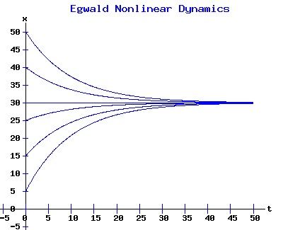
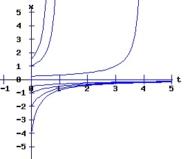
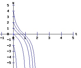
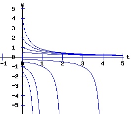
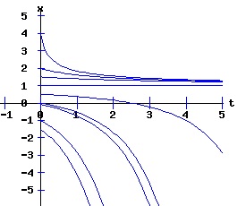
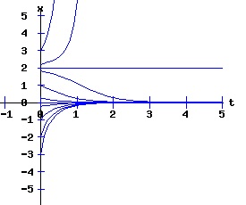
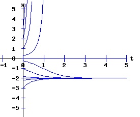
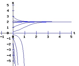
x(t) = e^k*t * x0.         (2)

The solution x(t) = e^k*t * x0 suggests that the population will grow or decay exponentially from its starting population, x0, at a rate depending on the magnitude of the parameter k.

Environments typically constrain the size of the population of an organism. Overcrowding and limited resources prevent an organism from increasing in number beyond some level. A slightly more realistic model includes a parameter, xe, representing this equilibrium population:

dx(t)/dt = k * (xe - x),   x(0) = x0 > 0.         (3)

If the population x at time t is less than xe, the population grows at the rate k times the difference (xe - x); if the population is greater than xe, the population decays at rate k times the difference (xe - x); if the population is xe, it remains at xe. This differential equation has the solution:

x(t) = xe + (x0 - xe) * e^(-k*t).         (4)

The next diagram illustrates some solution curves or trajectories, x(t), for various values of the initial population, x0, an equilibrium population of xe = 30, and a growth rate k = .10.

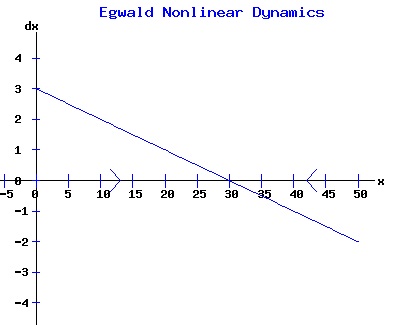
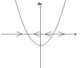
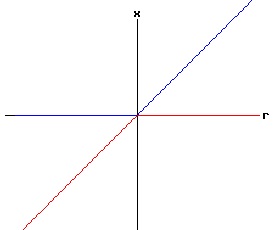
For populations much less than the environments sustainable level, the number of the organism grows rapidly, tapering off as the population reaches the equilibrium, xe = 30, level. Conversely, for populations much greater than the sustainable level, the number of the organism decreases rapidly with the rate of decay of the population tapering off as it reaches xe = 30.

The relation between the change in the population, dx, as a function of the population level, x, as described by equation (3) is:

dx = k * (xe - x),   x > 0         (5)

where dx is a function of x. The graph of this function is the phase diagram of the differential equation (3):

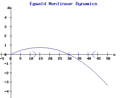
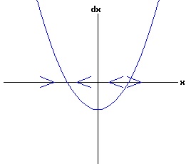
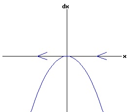
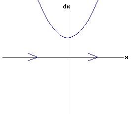
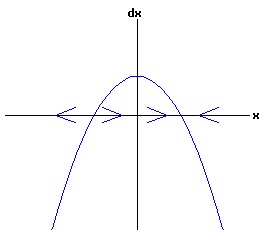
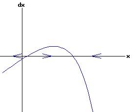
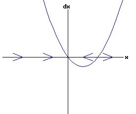
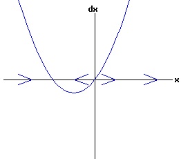
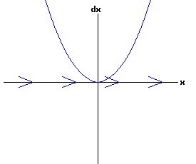
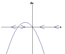
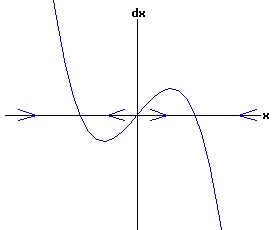
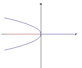
The change in population,dx, is positive for x < xe, and negative for x > xe, as indicated by the arrows on the x-axis. With any initial population, the population will adjust until the equilibrium population, xe, is attained. At this equilibrium, the available resources are just sufficient to maintain the population of the organism.

In the model above, the population grows most rapidly at small levels. If an organism needs to find a suitable mate to reproduce, the rate of growth should gradually increase with the size of the population, until environmental pressures reduce the rate of growth. In other words, one wants a differential equation with a quadratic phase diagram looking something like:

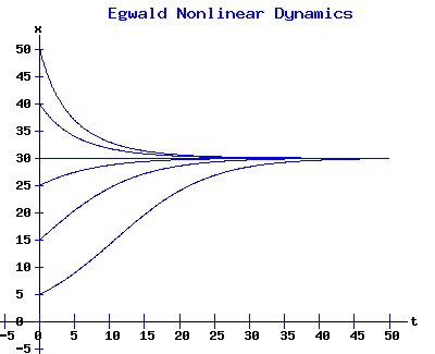
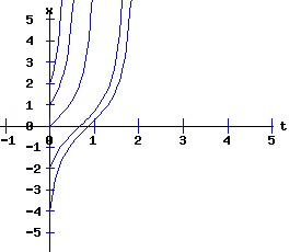
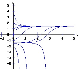
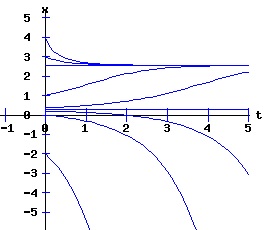
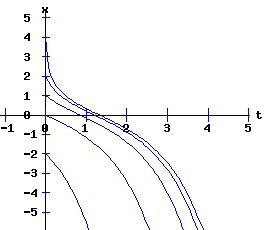
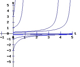
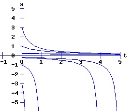
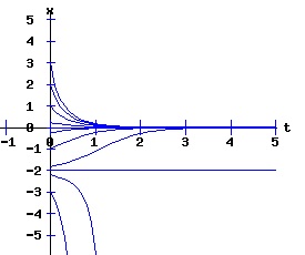
In this model, the rate of growth of the population has a maximum at x = 15, increasing from zero at x = 0, and decreasing to zero at xe = 30. For populations above xe = 30, the rate of growth is negative.

The well-known logistic differential equation:

dx(t)/dt = k * x * (1 - x / xe),   x(0) = x0 >= 0.         (6)

has these properties.

The relation between the change in the population, dx, as a function of the population level, x, as described by equation (6) is:

dx = k * x * (1 - x / xe),   x >= 0.         (7)

Graphing dx as a function of x yields the phase diagram above when xe = 30. If the initial population x0 = 0, the population will remain at 0 over time. In other words, xe = 0 is also an equilibrium along with xe = 30.

The next diagram illustrates some solution curves, x(t), for various values of the beginning population x0, an equilibrium population of xe = 30, and a growth rate k = .15.

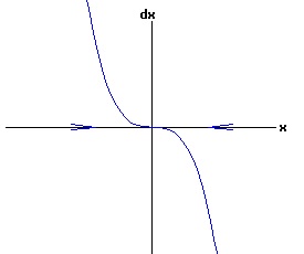
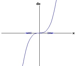
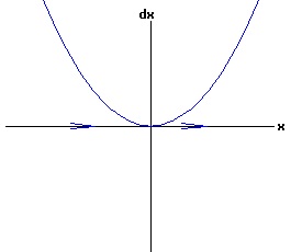
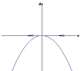
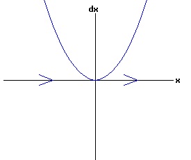
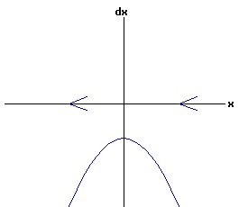
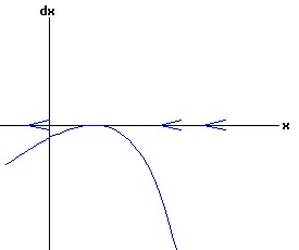
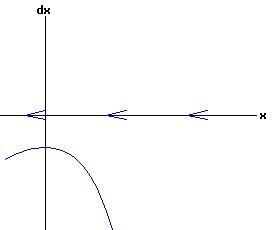
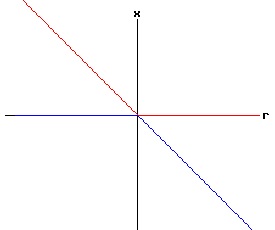
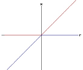
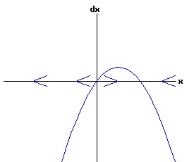
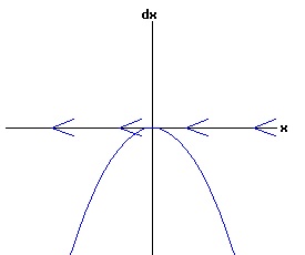
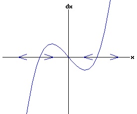
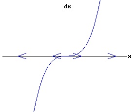
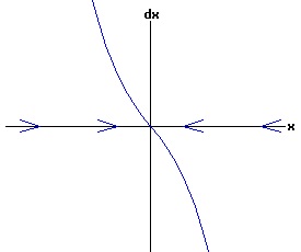
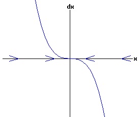
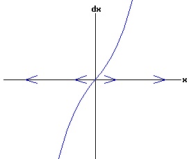
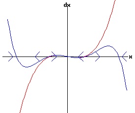
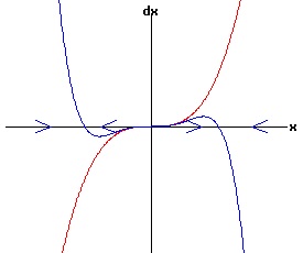
The general solution of the logistic differential equation is:

x(t) = xe / (1 - e^{(-k * t)} * (x0 - xe) / x0).         (8)

The set of all curves for specific values of xe and k are a one-parameter family of curves in the parameter x0, also called the integral curves of the differential equation (6). Equation (6) could also be considered as a one-parameter family in k, a one-parameter family in xe, a two-parameter family in k and xe, etc.

One Dimensional Differential Equations

The logistic equation is an example of a one dimensional differential equation. The general form of a one dimensional differential equation with a parameter r is:

dx / dt = f(x, r),   x(0) = x0.         (9)

If the function f is linear in x, the differential equation (9) is called linear; if the function f is nonlinear in x, it is called nonlinear.

While the solution of the nonlinear logistics differential equation can be represented explicitly by equation (8), determining the explicit solution of most nonlinear differential equations is very difficult or impossible. Consequently, the geometric properties of the function f are investigated to obtain qualitative information about the solution to the differential equation (9).

Fixed Points and Stability

For a specific value of the parameter r = r1, write:

dx / dt = f(x, r1) = f(x).         (10)

A fixed point of f is a number x^* such that:

f(x^*) = 0.         (11)

A fixed point x^* can also be called an equilibrium point (i.e. xe above), a critical point, a stationary point, or a rest point.

A fixed point x^* is stable if all trajectories starting "sufficiently close" to x^* stay "close" to x^*. The fixed point x^* is asymptotically stable if it is stable and trajectories starting "sufficiently close" to x^* eventually approach (decay) to x^* as t → ∞. A fixed point that is not stable is called unstable.

Linear Stability Analysis

One can analyze the local stability of the differential equation (10) about a fixed point by examining the first derivative of the function f with respect to x evaluated at x^*:

λ = f'(x^*).         (12)

The slope of f at the fixed point x^* determines the stability of (10).

The nonlinear process determined by the function f is stable at x^* if:

λ = f'(x^*) < 0;

the nonlinear process is unstable at x^* if:

λ = f'(x^*) > 0.

If λ ≠ 0, x^* is called a hyperbolic fixed point.

The stability of the process must be examined for each situation if:

λ = f'(x^*) = 0.

If λ = 0, x^* is called a non-hyperbolic fixed point.

Example: Logistic Equation Stability

The logistic equation (6) for k = 0.15 and xe = 30 is:

dx(t)/dt = f(x, 0.15)= f(x) = 0.15 * x * (1 - x /30).         (13)

Differentiating f with respect to x:

f'(x) = 0.15 * (1 - 2 * x / 30).         (14)

At x^* = 0:

λ = f'(0) = 0.15 > 0,

so the logistic process is unstable at x^* = 0.

At x^* = 30:

λ = f'(30) = -0.15 < 0,

so the logistic process is stable at x^* = 30.

Both fixed points are hyperbolic.

Examples of Non-Hyperbolic Fixed Points

Non-hyperbolic fixed points can be stable, unstable, or half-stable (unstable). A fixed point is half-stable (unstable) if trajectories converge to the fixed point on one side, but diverge from the fixed point on the other side. The following diagrams illustrate nonlinear processes with a fixed point x^* = 0, where f'(0) = 0.

One Dimensional Bifurcations.

A dictionary definition of bifurcation states: Division into two branches; the point of division; the branches or one of them. A nonlinear process experiences a qualitative change in its dynamics when the nature of its fixed points change. When a change in a parameter results in a qualitative change in the dynamics of a nonlinear process, the process is said to have gone through a bifurcation.

A one dimensional nonlinear dynamic process is modelled by the function f of two variables, x and r, where f is nonlinear in x, and r is a parameter. The differential equation governing the dynamics of the process is:

dx / dt = f(x, r),   x(0) = x0.         (15)

Bifurcations are classified by the way in which the fixed points of the function f change their number, location, form, and stability. It is convenient to consider normal forms for the different types of bifurcations, and the conditions under which the dynamic process described by equation (15) will experience a specific type of bifurcation.

Saddle-Node Bifurcation

The normal form of a saddle-node bifurcation is:

f(x, r) = a * (r - r_c) + b * (x - x^*)²,   a ≠ 0,   b ≠ 0.         (16)

The parameter is r; r_c and x^* are specific values.

Equation (16) has (x, r) = (x^*, r_c) as a fixed point since:

f(x^*, r_c) = a * (r_c - r_c) + b * (x^* - x^*)² = 0.         (17)

For specific values of the parameter r, r_c, and x^*, the roots of equation (16) are:

x₁ = x^* + sqrt( (-a / b) * (r - r_c) ),             

x₂ = x^* - sqrt( (-a / b) * (r - r_c) ).         (18)

Saddle-Node Conditions:

Saddle-Node Bifurcation Example: x^* = 0, r_c = 0.

For x^* = 0, and r_c = 0 equation (16) is:

f(x, r) = a * r + b * x².         (19)

The fixed points of f are:

x₁ = + sqrt( (-a / b) * r ),

x₂ = - sqrt( (-a / b) * r ).

Linearized stability:

Since:

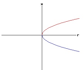
f(0, 0) = a * 0 + b * 0² = 0,

f_x(x, r) = 2 * b * x,

f_x(0, r) = 2 * b * 0 = 0,

the function f has a non-hyperbolic fixed point at x = x^* = 0, r = r_c = 0.

The stability of the dynamic process at each equilibrium point x₁, and x₂ depends on the values of f_x(x₁, r), and f_x(x₂, r), which depend on the signs of x₁ or x₂, and the coefficient b.

The phase diagram of equation (19) depends on the values of a, b, and r.

Type One Saddle-Node Bifurcation: Case a > 0, b > 0

In the following diagrams, a > 0, and b > 0. With r < 0, the phase diagram has two equilibria — one stable and one unstable. These two equilibria coalesce when r = 0, creating a half stable equilibrium. For r > 0, the equilibrium disappears because the discriminant of equation (18) is negative, resulting in complex number roots.

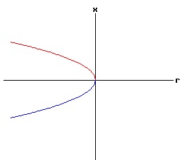
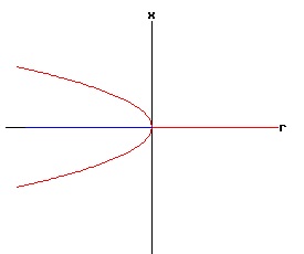
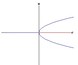
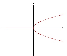
The following bifurcation diagram summarizes the behaviour of the equilibria for the saddle-node bifurcation. It shows the equilibria as a function of the parameter r. The blue curve represents the stable equilibria, while the red curve represents the unstable equilibria.

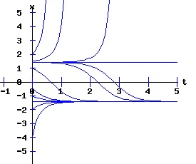
If r < 0, the nonlinear process has a negative (x < 0) stable equilibrium, and a positive (x > 0) unstable equilibrium. These equilibria coalesce at point, (r = 0, x = 0). This point, (x, r ) = (x^*, r_c) = (0, 0), is called the bifurcation point of the nonlinear dynamic process. For r > 0, the process diverges to +∞.

The next three diagrams contain graphs of the solution trajectories, x(t), for each case (r < 0, r = 0, r > 0) with some initial points, x(0) = x0.

With r < 0, the solution trajectories converge to -sqrt(2) for all initial points x(0) < sqrt(2). If x(0) = sqrt(2), x(t) = sqrt(2) for all t. With x(0) > sqrt(2), x(t) diverges to +∞.

With r = 0, x(t) converges to 0 for all x(0) <= 0. With x(0) > 0, x(t) diverges to +∞.

With r > 0, x(t) diverges to +∞ for all x(0).

Type Two Saddle-Node Bifurcation: Case a > 0, b < 0

Type Three Saddle-Node Bifurcation: Case a < 0, b > 0

Type Four Saddle-Node Bifurcation: Case a < 0, b < 0

Identifying Saddle-Node Bifurcations

The four types of saddle-node bifurcations can identify bifurcations for a differential equation of the form:

dx / dt = f(x, r),   x(0) = x0.         (20)

Example

Consider the differential equation:

dx / dt = f(x, r) = x - r * e^x,   x(0) = x0.         (21)

Step 1: Determine the non-hyperbolic fixed points.

Solve the next two equations for x = x^* and r = r_c:

Equation (22) implies r_c = x / e^x; equation (23) implies r_c = 1 / e^x. Together equations (22) and (23) imply the non-hyperbolic fixed point is:

(x, r) = (x^*, r_c) = (1, 1/e).         (24)

Step 2: Determine the non-zero a and b coefficients

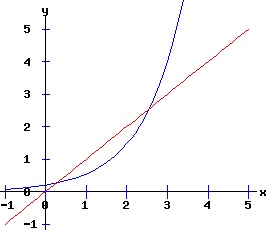
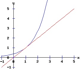
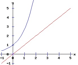
Since a < 0 and b < 0, the dynamic process of equation (21) has a Type Four saddle-node bifurcation at x = x^* = 1, r_c = 1/e, with two equilibria if r < r_c = 1/e, one equilibrium if r = 1/e, and no equilibria if r > 1/e.

The fixed points of equation (22) are the points of intersection of the curves y = x, and y = r * e^x.

The normal form of a differential equation with a saddle-node bifurcation is:

dx/dt = f(x, r) = a * (r - r_c) + b * (x - x^*)²,   x(0) = x0;   a ≠ 0,   b ≠ 0.         (27)

The dynamics of the differential equation:

dx / dt = f(x, r) = x - r * e^x,   x(0) = x0.         (28)

are qualitatively similar to the dynamics of the differential equation (27) with:

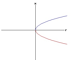
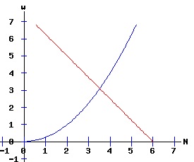
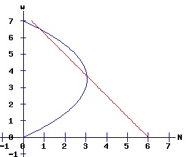
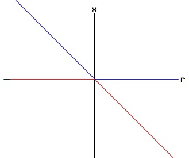
x^* = 1,   r_c = 1/e

a = -e,   b = -0.5

Example: Labour Market Bifurcation

The labour market has a demand and a supply schedule. The demand for labour, L_d, by firms is a decreasing function of the wage rate, w, while the supply of labour, L_s, by workers is an increasing function of the wage rate, w. The first diagram below illustrates these relationships, where the intersection of the L_d and L_s curves determine the equilibrium wage rate, w, and equilibrium number of workers hired, N. In the diagram of backward bending labour supply, the supply of labour function L_s, increases with the wage rate to a wage w, and decreases with any further increases in w.

Hans-Walter Lorenz describes this model's bifurcation in Nonlinear Dynamical Economics and Chaotic Motion (88-89), and Robert Crouch analyzes the validity of a backward bending labour supply schedule in Macroeconomics (40-42).

To illustrate the model geometrically, assume the functional forms:

L_d(w, r) = r - .8 * w,

L_s(w) = .25 * (3.5² - (w - 3.5)²),

where r is a parameter, and L_s(w) is the backward bending labour supply schedule in the diagram above.

The wage rate, w, adjusts according to the differential equation:

dw / dt = f(w, r) = L_d(w, r)   -   L_s(w),   w(0) = w0.

Step 1: Determine the non-hyperbolic fixed points.

Solve the next two equations for w = w^* and r = r_c:

The non-hyperbolic fixed point is:

(w, r) = (w^*, r_c) = (5.1, 6.5025).

Step 2: Determine the non-zero a and b coefficients

Since a > 0 and b > 0, the dynamic process of the labour market has a Type One saddle-node bifurcation at w^* = 5.1, r_c = 6.5025.

Transcritical Bifurcation

The normal form of a transcritical bifurcation is:

f(x, r) = a * (r - r_c) * (x - x^*) + b * (x - x^*)²,   a ≠ 0,   b ≠ 0.         (29)

The parameter is r; r_c and x^* are specific values.

After factoring (x - x^*) equation (29) becomes:

f(x, r) = (x - x^*) * [a * (r - r_c) + b * (x - x^*)],         (30)

revealing the roots of equation (29) as:

x₁ = x^*     

x₂ = x^* - (a / b) * (r - r_c).         (31)

Transcritical Conditions

Transcritical Bifurcation Example: x^* = 0, r_c = 0.

For x^* = 0, and r_c = 0 equation (29) is:

f(x, r) = a * r * x + b * x².         (32)

The fixed points of f are:

x₁ = x^* = 0,

x₂ = - (a / b) * r.

Linearized stability:

Since:

f(0, r) = 0 for all r,

f_x(x, r) = a * r + 2 * b * x,

f_x(0, r) = 0 for r = 0,

the function f has a non-hyperbolic fixed point at x = x^* = 0, r = r_c = 0.

The phase diagram of equation (32) depends on the values of a, b, and r.

Type One Transcritical Bifurcation: Case a > 0, b > 0

In the following diagrams, a > 0, and b > 0. With r < 0, the phase diagram has two equilibria — one stable at x = 0, and one unstable at x = -r > 0. These two equilibria coalesce when r = 0, creating a half stable equilibrium. For r > 0, the phase diagrams has two equilibria — one stable at x = -r < 0, and one unstable at x = 0.

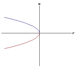
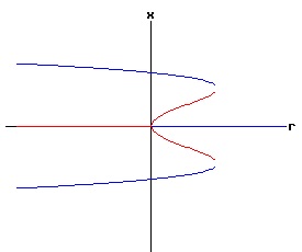
The following bifurcation diagram summarizes the behaviour of the equilibria for the transcritical bifurcation. It shows the equilibria as a function of the parameter r. The blue lines represent the stable equilibria, while the red lines represent the unstable equilibria.

If r < 0, the nonlinear process has a (x = 0) stable equilibrium, and a positive (x > 0) unstable equilibrium. These equilibria coalesce at point, (r = 0, x = 0). This point, (x, r ) = (x^*, r_c) = (0, 0), is called the bifurcation point of the nonlinear dynamic process. For r > 0, the nonlinear process has a negative (x < 0) stable equilibrium, and an unstable (x = 0) equilibrium.

The next three diagrams contain graphs of the solution trajectories, x(t), for each case (r < 0, r = 0, r > 0) with some initial points, x(0) = x0.

With r < 0, the solution trajectories converge to 0 for all initial points x(0) < -r. If x(0) = -r, x(t) = -r for all t. With x(0) > -r, x(t) diverges to +∞.

With r = 0, x(t) converges to 0 for all x(0) <= 0. With x(0) > 0, x(t) diverges to +∞.

With r > 0, the solution trajectories converge to -r < 0 for all initial points x(0) < 0. With x(0) > 0, x(t) diverges to +∞.

Type Two Transcritical Bifurcation: Case a > 0, b < 0

Type Three Transcritical Bifurcation: Case a < 0, b > 0

Type Four Transcritical Bifurcation: Case a < 0, b < 0

Identifying Transcritical Bifurcations

The four types of transcritical bifurcations can identify transcritical bifurcations for a differential equation of the form:

dx / dt = f(x, r),   x(0) = x0.         (33)

Example: Neoclassical Economic Growth

Consider the Solow Growth Model described in Economic Growth by Henry Wan (32-62), and in Nonlinear Dynamical Economics and Chaotic Motion by Hans-Walter Lorenz(90-92).

An economy produces a homogeneous good Y using capital K and labour L according to the production function Y = P(K, L). The labour force grows exponentially as dL/dt = n * L; the capital stock depreciates as dK/dt = μ * K, implying gross investment is I(t) = dK/dt + μ * K(t). If consumption is C(t), the economy's income identity is Y(t) = C(t) + I(t).

Dividing the variables Y, K, I, and C by L yields the per capita variables y, k, i, and c.

Using per capita variables, the production function becomes:

y = P(K/L, 1) = p(k),         (34)

the economy's income identity is:

y(t) = c(i) + i(t),         (35)

the gross investment identity is:

i(t) = (dK/dt)/L + μ * k(t),

where the rate of change of capital per worker is:

dk/dt = d(K/L)/dt = (dK/dt)/L - (dL/dt)/L * (K/L), so

(dK/dt)/L = dk/dt + n * k.

Consequently, the gross investment identity is:

i(t) = dk/dt + (μ + n) * k.         (36)

Using equations (34), (35), and (36), the fundamental differential equation of neoclassical economic growth is:

p(k(t)) - (μ + n) * k(t) = c(t) + dk(t)/dt.         (37)

If the economy's saving rate is s, per capita consumption is:

c(t) = (1 - s) * p(k).         (38)

Substituting (38) into (37) and rearranging results in the differential equation governing the growth of the economy's per capita capital stock:

dk/dt = s * p(k) - (μ + n) * k(t).         (39)

To illustrate this model geometrically, assume that the production function p(k) has the functional form:

y = p(k) = β * ln(1 + k),   β > 0.         (40)

(Note: This results in the Solow Growth Model without the Inada condition that p'(0) = ∞.)

The differential equation governing the dynamic process is:

dk/dt = f(k, s) = s * (β * ln(1 + k)) - (μ + n) * k,   k >=0,   k(0) = k0,         (41)

with the savings rate, s, as the parameter.

Check the Transcritical Bifurcation Conditions

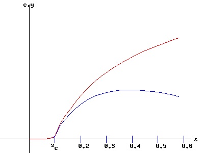
Since a > 0, and b < 0, the dynamic process of equation (41) has a Type Two transcritical bifurcation at s_c = (μ + n) / β, with one half (right) stable equilibrium if s = s_c, and two equilibria (unstable and stable) if s > s_c.

The equilibrium capital stock per capita, k, increases with the savings rate, s. Using Equations (38) and (40):

y = p(k) = β * ln(1 + k),

c = (1 - s) * p(k) = (1 - s) * y

one can graph the equilibrium income (output) per capita, y, and the equilibrium consumption per capita, c, as functions of the savings rate, s. For s < s_c, k, y, and c are zero. For s > s_c, equilibrium consumption per capita increases with the savings rate to a maximum and then decreases.

Specifying μ = 0.10, n = 0.05, and β = 1.5, s_c = (μ + n) / β = 0.10. The maximum consumption per capita occurs at s = 0.40.

Pitchfork Bifurcation

The normal form of a pitchfork bifurcation is:

f(x, r) = a * (r - r_c) * x + b * x³,   a ≠ 0,   b ≠ 0.         (45)

The parameter is r; r_c is a specific value.

Supercritical Pitchfork Bifurcation

In the normal form of a supercritical pitchfork bifurcation, the coefficient, b, in equation (45) is negative. Consequently, the cubic term stabilizes the dynamic process by pulling the trajectory of x(t) back toward x = 0.

Subcritical Pitchfork Bifurcation

In the normal form of a subcritical pitchfork bifurcation, the coefficient, b, in equation (45) is positive. Consequently, the cubic term destabilizes the dynamic process by driving the trajectory of x(t) toward infinity.

After factoring x equation (45) becomes:

f(x, r) = x * [a * (r - r_c) + b * x²],         (46)

revealing the roots of equation (45) as:

x₁ = 0,     

x₂ = + sqrt[-(a / b) * (r - r_c)],

x₃ = - sqrt[-(a / b) * (r - r_c)].

If -(a / b) * (r - r_c) >= 0 , x₂ and x₃ are real numbers.

Note that f is an odd function since:

f(-x, r) = -f(x, r),

and the function f does not have a transcritical bifurcation since:

f_x,x(0, r) = 0.

Pitchfork Conditions

Pitchfork Bifurcation Example: x^* = 0, r_c = 0.

For r_c = 0 equation (45) is:

f(x, r) = a * r * x + b * x³.         (47)

The fixed points of f are:

x₁ = 0,     

x₂ = + sqrt(-(a / b) * r),

x₃ = - sqrt(-(a / b) * r).

Linearized stability:

Since:

f(0, r) = 0 for all r,

f_x(x, r) = a * r + 3 * b * x²,

f_x(0, r) = 0 for r = 0,

the function f has a non-hyperbolic fixed point at x = x₁ = 0, r = r_c = 0.

The phase diagram of equation (47) depends on the values of a, b, and r.

Type One Pitchfork Bifurcation: Case a > 0, b > 0

In the following diagrams, a > 0, and b > 0. With r < 0, the phase diagram has three equilibria — in the order unstable (x₃), stable (x₁), and unstable (x₂). These three equilibria coalesce when r = 0 since x₁ = x₂ = x₃ = 0, resulting in one unstable equilibrium. For r > 0, x₂ and x₃ become pure imaginary numbers leaving one stable equilibrium at x₁ = 0.

Type Two Pitchfork Bifurcation: Case a > 0, b < 0

Type Three Pitchfork Bifurcation: Case a < 0, b > 0

Type Four Pitchfork Bifurcation: Case a < 0, b < 0

Identifying Pitchfork Bifurcations

The four types of pitchfork bifurcations can identify pitchfork bifurcations for a differential equation of the form:

dx / dt = f(x, r),   x(0) = x0.         (48)

Example: Kaldor Business Cycle Model

Consider the one dimensional version of Kaldor's Business Cycle Model described by Hans-Walter Lorenz in Nonlinear Dynamical Economics and Chaotic Motion (43-45, 92-94). Let the variable Y represent income, and y = Y - Y^* represent deviations from the stationary equilibrium income Y^*, with all the economy's goods subsumed into one good.

Savings, s(y), are a linear function of income

The income differential equation is:

dy / dt = α * (i(y, r)   -   s(y)),   y(0) = y0.         (49)

To illustrate the model geometrically, assume the functional forms:

i(y, r) = r * tanh(β * y),         (50)

s(y) = s * y,         (51)

where r is the parameter, and β and s are empirically determined coefficients.

The differential equation governing the dynamic process with α = 1 is:

dy /dt = f(y, r) = r * tanh(β * y)   -   s * y,   y(0) = y0.         (52)

Check the Pitchfork Bifurcation Conditions

Since a > 0, and b < 0, the dynamic process of equation (52) has a Supercritical bifurcation —
a Type Two pitchfork bifurcation at y = 0 , r_c = s / β,

Subcritical Pitchfork Bifurcation Revisited

The normal form of a subcritical pitchfork bifurcation is:

dx / dt = f(x, r) = a * r * x + x³.         (53)

The cubic term destabilizes the dynamic process by driving the trajectory of x(t) toward infinity.

Stabilized Subcritical Pitchfork Bifurcation

dx / dt = f(x, r) = a * r * x + x³ - x⁵.         (54)

The fixed points of f(x, r) in (53) are:

x₁ = 0,

x₂ = (1/2)*sqrt(2+2*sqrt(1+4*a*r)),

x₃ = -(1/2)*sqrt(2+2*sqrt(1+4*a*r)),

x₄ = (1/2)*sqrt(2-2*sqrt(1+4*a*r)),

x₅ = -(1/2)*sqrt(2-2*sqrt(1+4*a*r)).

Linearized stability

Since:

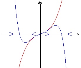
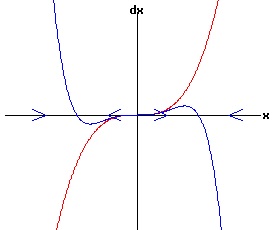
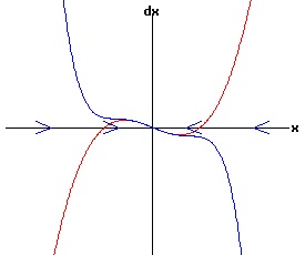
f(0, r) = 0 for all r,

f_x(x, r) = a * r + 3 * x² - 5 * x⁴,

f_x(0, r ) = 0 for r = 0,

the function f has a non-hyperbolic fixed point at x = x₁ = 0, r = r_c = 0.

Subcritical Pitchfork Bifurcation: Case a = 1 > 0

The following diagrams display the phase diagrams for equation (53) in red, and the phase diagrams for equation (54) in blue.

With r < -.25, equation (54) only has a stable fixed point at x₁ = 0. The other fixed points are complex numbers.

With -.25 <= r < 0, all fixed points are real with x₃ < x₅ < 0 < x₄ < x₂

With r = 0, x₁ = x₂ = x₃ = 0, and x₅ < 0 < x₄.

With r > 0, x₃ < 0 < x₂, while x₄ and < x₅ are complex numbers.

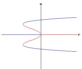
Subcritical Pitchfork Bifurcation: Case a = -1 < 0

The following diagrams display the phase diagrams for equation (53) in red, and the phase diagrams for equation (54) in blue.

dx = a * r * x + x3   and   dx = a * r * x + x3 - x5
r = -.5,	r = 0
Pitchfork Bifurcation Phase Diagrams

dx = a * r * x + x3   and   dx = a * r * x + x3 - x5
r = .1	r = .5
Pitchfork Bifurcation Phase Diagrams

dx = a * r * x + x3	dx = a * r * x + x3 - x5
Subcritical Pitchfork Bifurcation Diagrams

References.

• Burden, Richard L. and J. Douglas Faires. Numerical Analysis. 6th ed. Pacific Grove: Brooks/Cole, 1997.
• Demmel, James W. Applied Numerical Linear Algebra. Philadelphia: Siam, 1997.
• Devaney, Robert L. An Introduction to Chaotic Dynamical Systems. Menlo Park, CA: Benjamin/Cummings, 1986.
• Intriligator, M. D. Mathematical Optimization and Economic Theory. Englewood Cliffs: Prentice-Hall, 1971.
• Kaplan, Wilfred. Ordinary Differential Equations. Reading: Addison-Wesley, 1958.
• Lipschutz, Seymour. Linear Algebra. New York: Schaum McGraw-Hill, 1968.
• Lorenz, Hans-Walter. Nonlinear Dynamical Economics and Chaotic Motion. Berlin: Springer-Verlag, 1993.
• Mathews, John H. and Kurtis D. Fink. Numerical Methods Using MATLAB. 3rd ed. Upper Saddle River: Prentice Hall, 1999.
• Nagata, K. Wayne. Nonlinear Dynamics and Chaos: Mathematics 345 Lecture Notes. Vancouver: University of B.C., 2006
• Press, William H., Brian P. Flannery, Saul A. Teukolsky, and William T. Vetterling. Numerical Recipes: The Art of Scientific Computing. Cambridge: Cambridge UP, 1989.
• Strang, Gilbert. Linear Algebra and Its Applications. 3d ed. San Diego: Harcourt, 1976.
• Strogatz, Steven H. Nonlinear Dynamics and Chaos. Cambridge MA: Perseus, 1994.
• Wan, Henry Y. Jr. Economic Growth. New York: Harcourt, 1971.
• Watkins, David S. Fundamentals of Matrix Computations. New York: John Wiley, 1991.