
|
|
|
|
|
|
|
|
|
|
        
|
|
Egwald Mathematics: Nonlinear Dynamics:
Egwald's popular web pages are provided without cost to users.
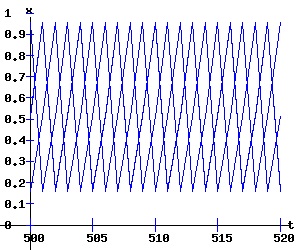
introduction | logistic map | fixed points | linearized stability analysis | bifurcation analysis The Logistic Map and Chaos: Introduction Introduction One can use the one-dimensional, quadratic, logistic map to demonstrate complex, dynamic phenomena that also occur in chaos theory and higher dimensional discrete time systems. The Logistic Map The logistic interative map with parameter r is: xt+1 = f(xt, r) = r * xt * (1 + xt), x0 = x0 >= 0. (1) For r values in excess of 3.57, the orbits x(t, x0) = {x0, x1, x2, ... } depend crucially on the initial condition x0. Slight variations in x0 result in dramatically different orbits, an important characteristic of chaos. Fixed Points Fixed points of f satisfy: f(x, r) = r * x * (1 - x) = x. (2) Thus the fixed points of f are the roots of the quadratic equation: r * x 2 - (r - 1) * x = x * (r * x - (r - 1)) = 0, (3) which are:
x1 = 0, The fixed point x2 is non-negative if r >= 1. Linearized Stability Analysis One can analyze the local stability of the difference equation (1) by examining the partial derivative of f with respect to x evaluated at each fixed point x*: λ = fx(x*, r) = r * (1 - 2 * x*). (5) where λ is called the multiplier or eigenvalue. Substituting x1 and x2 into (5) yields:
λ1 = r * (1 - 2 * x1) = r, If r > 1 → λ1 > 1 → x1 = 0 is unstable (repeller); if 1 < r < 3 → 1 > λ2 > -1 → x2 = (r - 1) / r is stable (attractor). Bifurcation Analysis When a change in a parameter results in a qualitative change in the dynamics of a nonlinear process, the process is said to have gone through a bifurcation. When r = 1 → λ1 = λ2 = 1 & x1 = x2 = 0 → (x*, rc) = (0 , 1) is a non-hyperbolic fixed point. In fact, it is a transcritical bifurcation point of the mapping f. Check the transcritical bifurcation conditions at (x*, rc) = (0, 1)
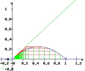
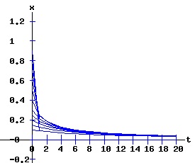
The transcritical bifurcation conditions are confirmed. Transcritical Bifurcation: r = 1 The following diagrams display the phase diagrams and solution trajectories of x(t, x0) for the discrete time, nonlinear dynamic process. At r = 1, the process undergoes a transcritical bifurcation with x1 switching from attractor to repeller. Meanwhile, the fixed point x2 turns positive and becomes an attractor, as can be seen in the diagrams for r = 2.
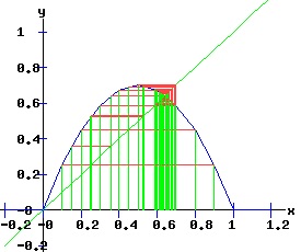
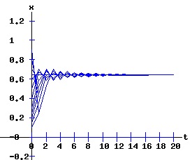
Period Doubling Bifurcation: r = 3 When r = 3 → λ2 = -1 & x2 = 2 / 3 → (x*, rc) = (2 / 3 , 3) is a non-hyperbolic fixed point. In fact, it is a period doubling (supercritical flip) bifurcation point of the mapping f. Check the period doubling bifurcation conditions at (x*, rc) = (2 / 3, 3)
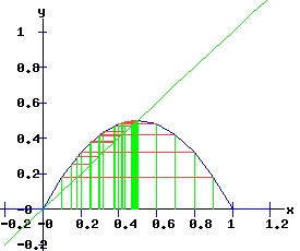
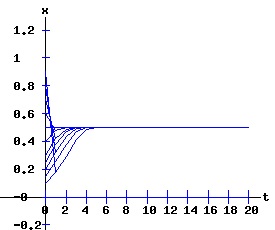
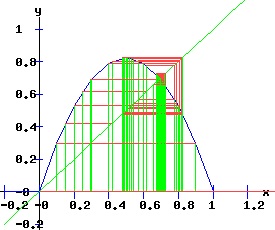
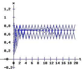
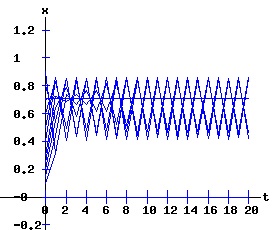
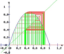
The period doubling bifurcation conditions are confirmed. Since c < 0 in expression F4, the fixed point x2 flips from being an attractor to being a repeller. Meanwhile, two stable fixed points of the second-order map f2 emerge that bracket the unstable x2. The trajectory xt switches between the two attracting fixed points of f2. The following diagrams display the phase diagrams and solution trajectories of x(t, x0) for the discrete time, nonlinear dynamic process. At r = 3, the f map undergoes a period doubling (flip) bifurcation with x2 switching from attractor to repeller. Meanwhile, two stable fixed points x3 and x4 of the second order map, f2 emerge.
The Second Order Map of f (f2) Associated with the logistic map: xt+1 = f(xt, r) = r * xt * (1 + xt), x0 = x0 >= 0. is the second order map f2 given by:
xt+2 = f(xt+1, r) = f (f(xt, r), r ) = r * (r * xt * (1 + xt)) * (1 + (r * xt (1 + xt))), or The partial derivative of f2 with respect to x is: fx2(x, r) = -4 * r3 * x3 + 6 * r3 * x2 - 2 * (r3 + r2) * x + r2. (8) Fixed points of (7) satisfy: f2(x, r) = -r3 * x4 + 2 * r3 * x3 - (r3 + r2) * x2 + r2 * x = x. (9) The fixed points of f2 are:
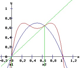
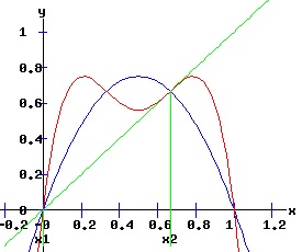
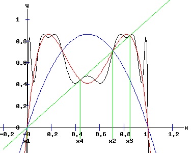
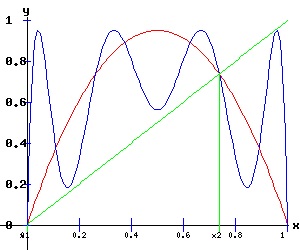
whose multipliers are: λi2 = fx2(xi, r). The first two fixed points of f2are also fixed points of f. The following graphs display the phase diagrams of f in blue and f2 in red. The stable fixed points x3 and x4 of f2 emerge as r increases past 3. At r = 3, f2 has a fixed point of multiplicity three (ie x2 = x3 = x4 = 2 / 3). For r > 3, x3 and x4 bracket x2, and establish the period-2 cycle seen in the above trajectory diagram for r = 3.3. Eventually, these period-2 fixed points become unstable, and undergo flip bifurcations with respect to f4, the period doubling map of f2.
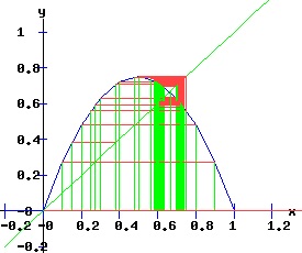
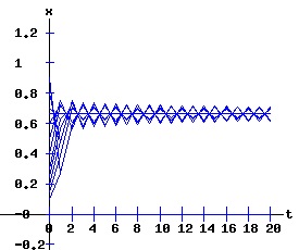
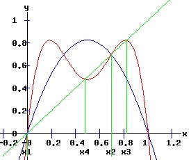
Second Order (f2) Flip Bifurcation : r = 1 + sqrt(6) When rc = 1 + sqrt(6) → x3 = 0.85 & x4 = 0.44 and λ23 = -1 & λ24 = -1 → x3 & x4 non-hyperbolic fixed points of f2. In fact, they are period doubling (supercritical flip) bifurcation points of the mapping f2. Check the period doubling bifurcation conditions at (x3,4, rc) for f2:
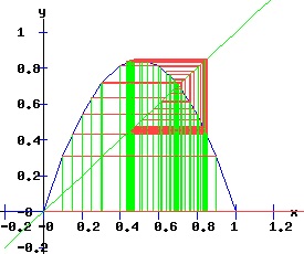
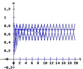
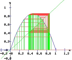
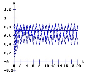
The period doubling bifurcation conditions are confirmed. Since c < 0 in the F4 expressions, the fixed points x3 and x4 flip from attractors to repellers. Meanwhile, four stable fixed points of the fourth-order map f4 emerge bracketing the unstable x3 and x4. The following diagrams display the phase diagrams and solution trajectories of x(t, x0) for the discrete time, nonlinear dynamic process. At r = 1 +sqrt(6) = 3.449489742, f2 undergoes a period doubling (flip) bifurcation with x3 and x4 switching from attractors to repellers. The trajectory xt switches between the four attracting fixed points of f4, creating a stable four-cycle.
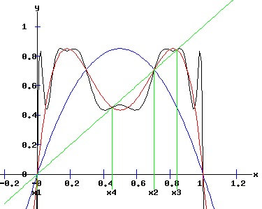
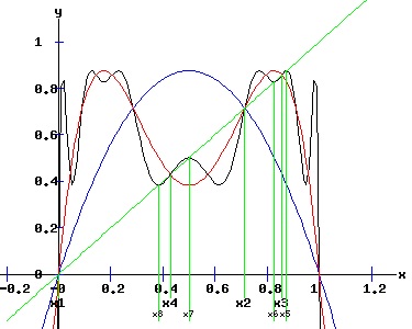
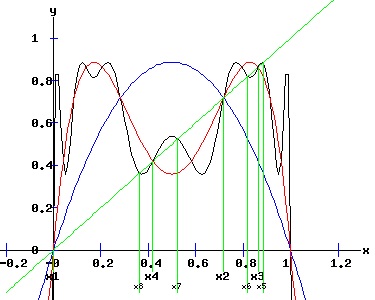
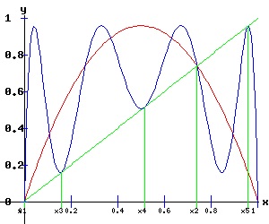
The Fourth Order Map of f (f4) Associated with the logistic map: xt+1 = f(xt, r) = r * xt * (1 + xt), x0 = x0 >= 0. is the fourth order map f4 given by: xt+4 = f4(xt, r) = f ( f ( f ( f (xt, r), r ), r ), r ) = f2 ( f2 (xt, r), r ) ), a polynomial in x of degree 16. Consequently, the 4th order map f4 has 16 fixed points, most of which will be complex, except the four fixed points f4 shares with f2, and the 4 fixed points that emerge at r = 1 + sqrt(6), bracketing x3 and x4. The following graphs display the phase diagrams of f in blue, f2 in red, and f4 in black. After the f2 period doubling bifurcation, four stable fixed points of the fourth order map, f4 emerge, x5 and x6 bracketing x3, and x7 and x8 bracketing x4.
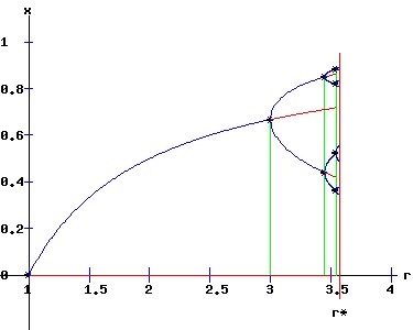
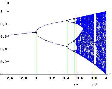
The bifurcation diagram below summarizes the fixed points and bifurcations of f, f2, and f4. The f map experiences a transcritical bifurcation at r = 1, and a period doubling bifurcation at r = 3. In turn, the f2 map undergoes a period doubling bifurcation at r = 1 + sqrt(6), while the f4 map undergoes a period doubling bifurcation a r = 3.54409. Stable fixed points of f, f2, and f4 are in blue, while unstable fixed points are in red.
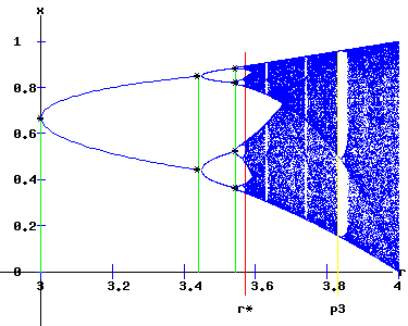
Period Doubling Cascade As r increases, period doublings occur as f, f2, f4, f8, . . . bifurcate at r1 = 3, r2 = 3.449, r3 = 3.54409, r4 = 3.5644, . . .. These {2n} cycles of {f2n} and {rn} sequences follow the Feigenbaum rule: δ = (rn - rn-1) / (rn+1 - rn) → 4.6692 as n → ∞. In the limit as n → ∞, rn → r* = 3.570. Logistic Map Bifurcation Diagram The bifurcation diagram shows the set of stable fixed points, {x*(r)}, as a function of the parameter r for the logistics map: xt+1 = f(xt, r) = r * xt * (1 + xt), x0 = x0 >= 0. (10) For 1 < r < r*, the period doubling cascade of the sequence of maps {f2n} determines the attracting fixed points.
For r* < r <= 4, the band of stable fixed points expands to cover the entire vertical [0, 1] interval at r = 4. For many values of r in the horizontal [r*, 4] interval, the orbit: {xt+1 = f(xt ,r), x0 = x0} exhibits aperiodic — chaotic — behaviour . Also for r in this [r*, 4] interval, periodic windows appear. The widest window at r = p3 = 1 + sqrt(8) is the period 3 window. As r increases from r* to p3, period 6 and period 5 windows also appear. Depending on the value of the parameter r, orbits of the logistic map appear orderly or chaotic. The Third Order Map of f, f3 For r < p3, the f3 map has two unstable fixed points it shares with the f map. At r = p3 = 1 + sqrt(8), three fixed points emerge, where the graph of the f3 map has 3 points of tangency with the y = x line. Here, the f3 map undergoes a triple saddle-node bifurcation.
Saddle-Node Bifurcation of f3: r = 1 + sqrt(8) = 3.8284 The following table verifies the triple saddle-node bifurcation of the f3 map at the fixed points x3 = 0.15999288, x4 = 0.51435528, and x5 = 0.9563178.
The f3 map undergoes Type Three (a < 0, b > 0) saddle-node bifurcations at x3 and x4, and a Type Two (a > 0, b < 0) saddle-node bifurcation at x4. One can see the effects of these bifurcations in the diagram below. At r = 3.839, x3, x4, and x5 have each split into a pair of fixed points, one stable and the other unstable.
Third Order Flip Bifurcation : r = 3.8414991 At r = 3.8414991, x3, x4, and x5 flip from attractors to repellers. The f3 map undergoes a flip bifurcation. Pairs of stable fixed points of the f9 emerge bracketing x3, x4, and x5.
When rc = 3.8414991 → x3 = 0.14872043, x4 = 0.48634402 x5 = 0.953596008 and λ33,4,5 = -1 → x3,4,5 are non-hyperbolic fixed points. In fact, they are period doubling (supercritical flip) bifurcation points of the mapping f3. Check the period doubling bifurcation conditions at (x3,4,5, rc) for f3:
The period doubling bifurcation conditions are confirmed. The control of the pairs of stable fixed points of the f3 map that bracket the unstable x3, x4, and x5 fixed points of f3 of the orbits {xt} is evident in the next diagram.
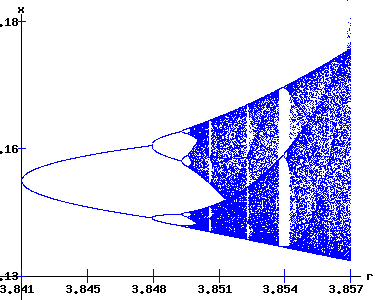
The f3 Period Doubling Cascade As r increases, period doublings occur at r1 = p31, r2 = p32, r3 = p33, .... as f3, f9, f27, . . . flip bifurcate. The orbit diagram around the fixed point x3 of f3 in the region 3.8414991 < r < 3.857 and 0.13 < x < 0.18 shows the period doubling cascade of the sequence of maps {f3n} determining the attracting fixed points of the specific f3n map for p3n <= r < p3n+1. In the limit as n → ∞, p3n → p3*.
The intermittent emergence of order and chaos revealed in the above miniature orbit diagram for r in the interval [3.8414991, 3.857] mirrors the pattern of the complete orbit diagram for r in the interval [3, 4] available below.
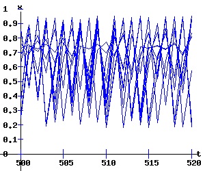
As r converges to 4, the {xt} orbits become increasingly chaotic, evident in the diagrams for f and f3, and the solution trajectory.
For r > 4, most trajectories leave the [0, 1] vertical interval. Interactive Logistic Map Diagrams Click to pop a new window with some interactive logistic map diagrams. Definitions of Chaos "Stochastic behavour in a deterministic system." "Chaos is aperiodic long-term behavour in a deterministic system that exhibits sensitive dependence on initial conditions" (Strogatz 323). Let V be a set. The mapping f: V → V is said to be chaotic on V if: References.
|
|||||||||||||||||||||||||||||||||||||||||||||||||||||||||||||||||||||||||||||||||||||||||||||||||||||||||
|

