Egwald Mathematics: Nonlinear Dynamics:

Trygve Haavelmo Growth Model

Continuous versus Discrete Time

by

Elmer G. Wiens

Egwald's popular web pages are provided without cost to users.
Please show your support by joining Egwald Web Services as a Facebook Fan:
Follow Elmer Wiens on Twitter:

introduction | continuous time | phase diagrams | discrete time | phase diagrams | bifurcation diagram
continuous versus discrete | references

The Trygve Haavelmo Growth Model

The Trygve Haavelmo growth model in A Study in the Theory of Economic Evolution. provides an example of the different dynamical behaviours arising from equivalent models expressed as either differential or difference equations. While the solution trajectories of the continuous time version of the model converge to its fixed point, the solution trajectories of the discrete time version may exhibit chaotic behaviour.

As described by Hans-Walter Lorenz in Nonlinear Dynamical Economics and Chaotic Motion (141-143), the one-dimensional Haavelmo (28-29) growth cycle model describes an economy's production of output as a function of the stock of capital (K) and the level of employment (N).

Continuous Time

Y = c * K^(1-a) * N^a,     0 < a < 1,   c > 0,         (1)

the differential equation governing the growth of employment is:

dN / dt = N * (α - β * N / Y),   N(0) = N0,     α, β > 0,         (2)

whose solution is a function N(t) = N(t, N0)) of time, t, and the initial condition, N(t=0) = N0.

Thus, the rate of growth of employment, dN/dt / N, is an increasing function of per capita income (output), Y / N.

Combining equations (1) and (2) yields:

dN / dt = f(N, α) = α * N - β / (c * K^(1-a)) * N^{(2 - a)},   N(0) = N0.         (3)

where α is the parameter of the differential equation (2) to be analyzed.

The Fixed Point

To find the fixed point, set f(N, α) = 0, and solve for N^*:

f(N, α) = α * N - β / (c * K ^(1-a)) * N^{(2 - a)} = 0, or

N^* = (α * c * K^(1-a) / β)^{1 / (1 - a)}.         (4)

Linear Stability Analysis

Evaluating the partial derivative of f with respect to N at the fixed point N^* yields:

f_N(N, α) = α - (2 - a) * (β / (c * K^{(1 - a)} * N^{(1 - a)}, and

f_N(N^*, α) = α * (a - 1) < 0,

since α > 0 and 0 < a < 1. Thus the nonlinear process determined by the function f is stable with the fixed point at N^*.

Phase Diagrams and Solution Trajectories

Particularize the continuous growth model by setting:

K = 3,     a = .3,     β = 1,     c = .9.

with parameter α and initial condition N(0) = N0.

The following diagrams show the phase diagrams and solution trajectories, N(t), for various initial conditions N(0), and two values of the parameter α.

Discrete Time

In the differential equation (3), replace the trajectory function N(t) by the trajectory orbit {N_t}, and the differential operator dN / dt with the finite difference N_t+1 - N_t to yield the difference equation:

N_t+1 - N_t = α * N_t - β / (c * K^(1-a)) * N_t^{(2 - a)},   N₀ = N0, or

    N_t+1 = (1 + α) * N_t - β / (c * K^{(1 - a)}) * N_t^{(2 - a)},   N₀ = N0.         (5)

This difference equation can be transformed by the transformation:

N_t = (K^{(1 - a)} * (1 + α) / β)^{1/(1 - a)} * x_t

to produce the equation:

x_t+1 = f(x_t, α) = (1 + α) * x_t * (1 - x_t^{(1 - a)}),   x₀ = x0 > 0.         (6)

The dynamics of equation (6) are qualitatively equivalent to those of the logistics equation (set r = (1 + α) and let a → 0). Moreover, f(0, α) = f(1, α) = 0, and f is one-humped and noninvertible.

Fixed Points

Fixed points of the discrete f map satisfy:

f(x, α) = (1 + α) * x * (1 - x^{(1 - a)}) = x,         (7)

which are:

x₁ = 0,

x₂ = [α/ (1 + α)]^{1/ (1 - a)}.         (8)

Linear Stability Analysis

The partial derivative of f with respect to x is:

f_x (x, α) = (1 + α) * (1 - (2 - a)) * x ^{(1 - a)}.        (9)

Evaluating f at its fixed points to obtain the multipliers:

λ₁ = f_x(0, α) = (1 + α), and

λ₂ = f_x(x₂, α) = (1 + α)*(1 - (2 - a) * α/ (1 + α) = 1 - α * (1 - a).

Since α > 0 → λ₁ > 1 → x₁ = 0 is a repeller.   If 0 < α < 2 / (1 - a) → 1 > λ₂ > -1 → x₂ is an attractor.

Phase Diagrams and Solution Trajectories

Particularize the discrete growth model by setting:

a = .3.

with parameter α and initial condition x₀ = x0.

The fixed point x₂ of f is an attractor in the range:

0 < α < 2 / (1 - a) = 2 / .7 = 2.8571.         (10)

At α = 2 / (1 - a) = 2 / .7, the f map undergoes a flip bifurcation, where x₂ switches from attractor to repeller.

The following diagrams show the phase diagrams and solution trajectory orbits, {x_t}, for various initial conditions x₀ and values of the parameter α.

The Second Order Map of f, denoted by f², is x_t+2 = f(x_t+1, α) = f (f(x_t, α), α ) = f²(x_t, α) .

The following graphs display the phase diagrams of f in blue and f² in red. The stable fixed points x₃ and x₄ of f² emerge as α increases past 2/.7. At α = 2 / .7 = 2.8571, f² has a fixed point of multiplicity three (ie x₂ = x₃ = x₄ = 2 / .7). For α > 2/.7, x₃ and x₄ bracket x₂, and establish the period-2 cycle seen in the above trajectory diagram for α = 3.2. Eventually, these period-2 fixed points become unstable, and undergo flip bifurcations with respect to f⁴, the period doubling map of f².

Second Order (f²) Flip Bifurcation

The following diagrams display the phase diagrams and solution trajectories of x(t, x0) for the discrete time, nonlinear dynamic process. At α = 3.48365646, f² undergoes a period doubling (flip) bifurcation with x₃ and x₄ switching from attractors to repellers. The trajectory x_t switches between the four attracting fixed points of f⁴, creating a stable four-cycle.

The Fourth Order Map of f, denoted by f⁴, is x_t+4 = f² (f²(x_t, α), α ) = f⁴(x_t, α) .

The following graph displays the phase diagrams of f in blue, f² in red, and f⁴ in black. The fixed points x₃ and x₄ of f² flip from attractor to repeller as α increases past 3.48365646. For α > 3.48365646, four stable fixed points of f⁴ emerge bracketing x₃ and x₄, and establish the period-4 cycle. Eventually, these period-4 fixed points become unstable, and undergo flip bifurcations with respect to f⁸, the period doubling map of f⁴.

Fourth Order (f⁴) Flip Bifurcation

The following diagrams display the phase diagrams and solution trajectories of x(t, x0) for the discrete time, nonlinear dynamic process. At α = 3.61271754, f⁴ undergoes a period doubling (flip) bifurcation with x₅, x₆, x₇, and x₈ switching from attractors to repellers. The trajectory x_t switches between the eight attracting fixed points of f⁸, creating a stable eight-cycle.

The following graph displays the phase diagrams of f in blue, f⁴ in red, and f⁸ in black. The fixed points x₅, x₆, x₇, and x₈ of f⁴ flip from attractor to repeller as α increases past 3.61271754. For α > 3.61271754, eight stable fixed points of f⁸ emerge bracketing x₅, x₆, x₇, and x₈, and establish the period-8 cycle. Eventually, these period-8 fixed points become unstable, and undergo flip bifurcations with respect to f¹⁶, the period doubling map of f⁸.

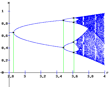
Period Doubling Cascade

As α increases, period doublings occur as f, f², f⁴, f⁸, . . . bifurcate at α₁ = 2/.7, α₂ = 3.4837, α₃ = 3.6127, α₄ = . . ..

Bifurcation Diagram

The intermittent emergence of order and chaos is revealed in the orbit diagram below, for α (called r) in the interval [2.8, 4].

{x_t+1 = f(x_t ,α), x₀ = x0}

exhibits aperiodic — chaotic — behaviour, as α increases, with periodic windows appearing. These dynamics are qualitatively similar to those observed with the logistics map.

Continuous versus Discrete Time Dynamics.

The table below shows how the economy's levels of employment and output increases in a stable manner with α in the continuous time model. However, in the discrete time model, these levels of employment and output cycle and exhibit chaotic dynamics as α increases.

References.

• Haavelmo, Trygve. A Study in the Theory of Economic Evolution. Amsterdam: North-Holland, 1954.
• Lorenz, Hans-Walter. Nonlinear Dynamical Economics and Chaotic Motion. Berlin: Springer-Verlag, 1993.