Egwald Mathematics: Nonlinear Dynamics:

Bifurcations and Two Dimensional Flows

by

Elmer G. Wiens

Egwald's popular web pages are provided without cost to users.
Please show your support by joining Egwald Web Services as a Facebook Fan:
Follow Elmer Wiens on Twitter:

bifurcation definition | introduction | prototype bifurcations
saddle-node | transcritical | pitchfork | hopf bifurcation
two parameter bifurcations | monkey saddle | global bifurcations
cycle saddle-node | infinite period | homoclinic bifurcation
references

Definition: Bifurcation

A differential equation system undergoes a bifurcation when a qualitative change in its orbit structure appears, as one or more parameters of the dynamical system are changed. Bifurcation theory studies structurally unstable dynamical systems.

Dynamic stability refers to perturbations in the phase space—the stability of fixed points and limit cycles. Structural stability refers to perturbations in the function space—the topological stability of orbit structures (Medio 55-69).

Introduction:

Describe the dynamics of a two dimensional, continuous time process by a pair of differential equations and initial conditions:

dx / dt = f(x, y, α),         (1)

dy / dt = g(x, y, α),         (2)

  x(t₀) = x0,   y(t₀) = y0,       (3)

whose solution, x(t, α) and y(t, α), is a pair of continuous functions of time t, that also depend on the parameter, α.

One Parameter Prototype Bifurcations

Structurally unstable dynamic systems can be classified according to the number of parameters that appear in the differential equations describing the system's dynamics. The following examples are one parameter systems, and are the two dimensional analogues to the one dimensional normal forms for one dimensional bifurcations.

The uncoupled differential equations for the saddle-node, transcritical, and pitchfork bifurcations have the form:

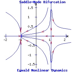
dx / dt = f(x, y, α) = f(x, α),         (4)

dy / dt = g(x,y, α) = g(y) = -y,         (5)

  x(t₀) = x0,   y(t₀) = y0,       (6)

Consequently, each system's fixed points occur along the x-axis. Furthermore, the solutions to the second differential equations have the exponential form:

y(t) = e^-t * y₀

with solution trajectories decaying to the x-axis through time.

Example: Saddle-Node Bifurcation

The saddle-node prototype system is:

dx / dt = f(x, y) = a * α + b * x²,         (7)

dy / dt = g(x, y) = -y,                   (8)

This system's fixed points are:

(x₁, y₁) = ( sqrt( (-a / b) * α ), 0 ), 

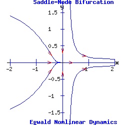
(x₂, y₂) = ( -sqrt( (-a / b) * α ), 0 ).

Letting a = 1, b = 1, the x-component of a fixed point is a real number if α <= 0.

The Jacobian matrix is:

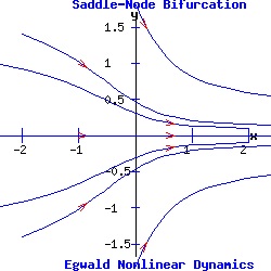
Thus, p = trace(J) = -1 + 2 * b * x, and q = det(J) = -2 * b * x. Let a = 1, b = 1. For α = -1, the first fixed point is an attractor with eigenvalues μ₁ = -1 and μ₂ = -2; meanwhile, the second fixed point is a saddle point with eigenvalues μ₁ = 2 and μ₂ = -1. For α = 0, the origin is a double fixed point with eigenvalues μ₁ = 0 and μ₂ = -1, attracting initial points with a non-positive y-component. For α > -1, there are no real fixed points.

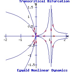
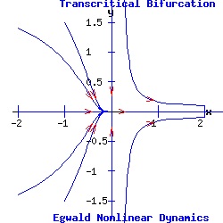
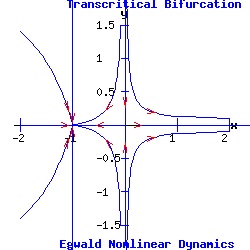
Example: Transcritical Bifurcation

The transcritical prototype system is:

dx / dt = f(x, y) = a * α * x + b * x²,         (9)

dy / dt = g(x, y) = -y,                     (10)

This system's fixed points are:

(x₁, y₁) = ( 0, 0 ), 

(x₂, y₂) = ( -(a / b) * α, 0 ).

The Jacobian matrix is:

Thus, p = trace(J) = -1 + a * α + 2 * b * x, and q = det(J) = -a * α - 2 * b * x. Let a = 1, b = 1. For α = -1, the first fixed point is an attractor with eigenvalues μ₁ = -1 and μ₂ = -1; meanwhile, the second fixed point is a saddle point with eigenvalues μ₁ = 1 and μ₂ = -1. For α = 0, the origin is a double fixed point with eigenvalues μ₁ = 0 and μ₂ = -1, attracting initial points with a non-positive y-component. For α = 1, the first fixed point, (x₁, y₁), is a saddle-node, and the second fixed point, (x₂, y₂), is an attractor.

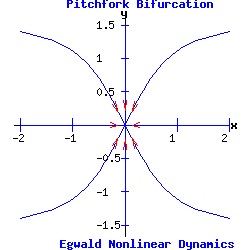
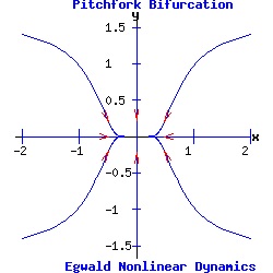
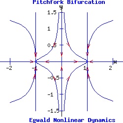
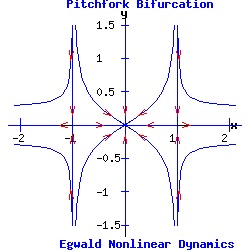
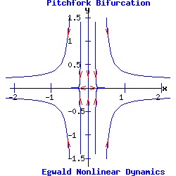
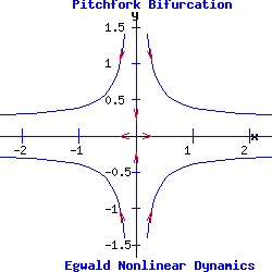
Example: Pitchfork Bifurcation

The pitchfork prototype system is:

dx / dt = f(x, y) = a * α * x + b * x³,         (11)

dy / dt = g(x, y) = -y,                     (12)

Supercritical Pitchfork Bifurcation

In the normal form of a supercritical pitchfork bifurcation, the coefficient b in equation (11) is negative. Consequently, the cubic term stabilizes the dynamic process by pulling the trajectory of x(t) toward the stable fixed point(s).

Subcritical Pitchfork Bifurcation

In the normal form of a subcritical pitchfork bifurcation, the coefficient b in equation (11) is positive. Consequently, the cubic term destabilizes the dynamic process by driving the trajectory of x(t) toward infinity.

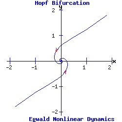
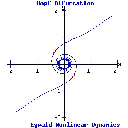
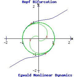
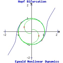
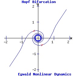
The heteroclinic line joining the two saddle points when α < 0 collapses as the saddle points collide when α passes through 0.

The Hopf Bifurcation

With the saddle-node, transcritical, and pitchfork bifurcations, the stable fixed point has p = trace(J) < 0, and q = det(J) > 0. Its eigenvalues are real and negative ( lie in the left half-plane). As α varies for the transcritical and pitchfork bifurcations, one eigenvalue becomes positive, turning the fixed point into a saddle-node.

With Hopf bifurcations, the fixed point's eigenvalues are complex conjugates, µ₁ and µ₂.

In a supercritical Hopf bifurcation, as the parameter α varies a stable node with Re(µ_{1, 2}) < 0 turns unstable with Re(µ_{1, 2}) > 0, while simultaneously a stable limit-cycle emerges.

In a subcritical Hopf bifurcation, as α varies an unstable node with Re(µ_{1, 2}) > 0 turns stable with Re(µ_{1, 2}) < 0, while simultaneously the unstable limit-cycle disappears.

Example: Supercritical Hopf Bifurcation

Consider the nonlinear system with functions f and g given by:

dx / dt = f(x, y) = - y + x * (α - (x² + y²)),

dy / dt = g(x, y) = x + y * (α - (x² + y²)).

This system has a fixed point at (x^*, y^*) = (0, 0).

The Jacobian matrix at the fixed point is:

Since p = trace(J) = 2 * α, and q = det(J) = α² + 1 > 0, the fixed point (0, 0) is a hyperbolic attractor with eigenvalues μ₁ = -1/2 + i and μ₂ = -1/2 - i if α = -.5 < 0; a hyperbolic repeller with eigenvalues μ₁ = 1 + i and μ₂ = 1 - i if α = 1 > 0; and a non-hyperbolic fixed point if α = 0. (See the topological classification of fixed points.)

As α increases past 0, the fixed point at the origin switches from attractor to repeller and a stable limit cycle (attractor) emerges for α > 0.

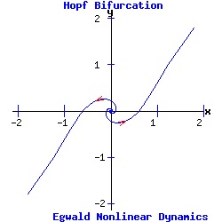
Example: Subcritical Hopf Bifurcation

Consider the nonlinear system with functions f and g given by:

dx / dt = f(x, y) = - y + x * (α + (x² + y²)),

dy / dt = g(x, y) = x + y * (α + (x² + y²)).

This system has a fixed point at (x^*, y^*) = (0, 0).

The Jacobian matrix at the fixed point is:

Since p = trace(J) = 2 * α, and q = det(J) = α² + 1 > 0, the fixed point (0, 0) is a hyperbolic attractor with eigenvalues μ₁ = -1 + i and μ₂ = -1 - i if α = - 1 < 0; a hyperbolic repeller with eigenvalues μ₁ = 1/2 + i and μ₂ = 1/2 - i if α = .5 > 0; and a non-hyperbolic fixed point if α = 0. (See the topological classification of fixed points.)

Although this Jacobian is the same as the Jacobian of the dynamic system with a supercritical Hopf bifurcation, the orbit structure revealed in the next diagram is topologically different from the supercritical orbit structure.

For α < 0, the unstable limit cycle (repeller) surrounds the attracting fixed point at the origin. As α increases past 0, the fixed point at the origin switches from attractor to repeller and the limit cycle disappears.

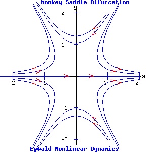
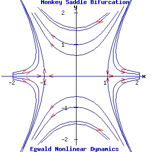
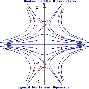
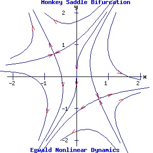
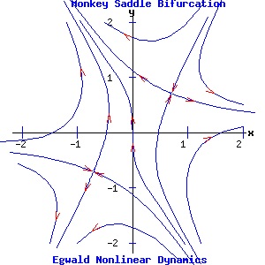
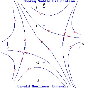
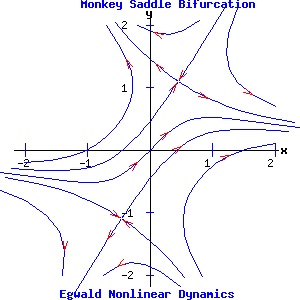
Two Parameter Bifurcations

Monkey Saddle Bifurcation

The differential equations controlling the dynamics of the monkey saddle and its bifurcations:

dx / dt = f(x, y) = x² - y² + α,

dy / dt = g(x, y) = -2 * x * y + β.

have two parameters, α and β.

The system's Jacobian matrix is:

α = 0, β = 0: the system has a double fixed point at the origin. Since the Jacobian evaluated at the origin has all zero entrees, p = trace(J) = 0, and q = det(J) = 0. Consequently, both eigenvalues are zero and the origin is a non-hyperbolic fixed point.

α = -1, β = 0: the fixed points are (1, 0) and (-1, 0). The Jacobian evaluated at either fixed point has p = 0 and q = -4. Consequently, the fixed points are saddle points, joined by a heteroclinic trajectory from (1, 0) to (-1, 0).

α = 1, β = 0: the fixed points are (0, 1) and (0, -1). The Jacobian evaluated at either fixed point has p = 0 and q = -4. Consequently, the fixed points are saddle points.

α = 0, β = -1: the fixed points are (-1/2*√2,  1/2*√2) and (1/2*√2,  -1/2*√2). The Jacobian evaluated at either fixed point has p = 0 and q = -4. Consequently, the fixed points are saddle points.

α = 0, β = 1: the fixed points are (1/2*√2,  1/2*√2) and (-1/2*√2,  -1/2*√2). The Jacobian evaluated at either fixed point has p = 0 and q = -4. Consequently, the fixed points are saddle points.

α = -1, β = 1: the fixed points are (1.0987, 0.4551) and (-1.0987, -0.4551). The Jacobian evaluated at either fixed point has p = 0 and q = -5.6569. Consequently, the fixed points are saddle points.

α = 1, β = 1: the fixed points are (0.4551, 1.0987) and (-0.4551, -1.0987). The Jacobian evaluated at either fixed point has p = 0 and q = -5.6569. Consequently, the fixed points are saddle points.

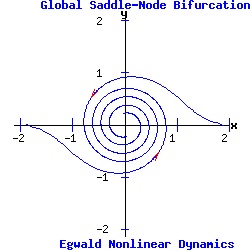
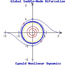
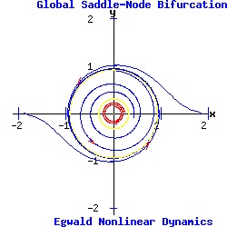
Global Bifurcations (Strogatz 260-265)

Global Bifurcations involve changes to the orbit structure of the dynamic system that leave the underlying fixed points and their topological stability properties unchanged.

Global Saddle-Node (Fold) Bifurcation

Express the system in polar coordinates, where r = distance of a point from the origin, and θ = the angle from the x-axis to the line joining the point to the origin, measured counterclockwise. The parameter α of the dynamic system:

dr / dt = α * r + r³ - r⁵,         (13)

d θ / dt = a + b * r²,         (14)

determines the global bifurcation. The system has a fixed point attractor at the origin. As α increases, a half-stable limit cycle appears, which splits into a smaller unstable limit cycle, and a larger stable limit cycle. In the example below with a = 2 and b = .1, the limit cycle appears with radius r = .70711 at the critical parameter value of α_c = -.25. For α = -.1 > α_c, the radii of the limit cycles are r₁ = .335711, and r₂ = .941965. As α increases, the fixed point at the origin continues as an attractor.

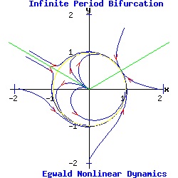
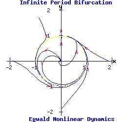
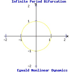
Equation (13) as a one dimensional system undergoes a type-two saddle-node bifurcation for r > 0.

Infinite-Period Bifurcation

In polar coordinates, the uncoupled system is:

dr / dt = r * (1 - r²),         (15)

d θ / dt = α - sin( θ ).         (16)

Equation (15) is a one dimensional system with stable fixed points at r₁ = -1, and r₂ = 1, separated by an unstable fixed point at the origin where r^* = 0 (type two pitchfork bifurcation).

Equation (16) is a one dimensional nonuniform oscillator, exhibiting the properties of a type one saddle-node bifurcation. When α > 1, counterclockwise flow varies with the value of θ, having a maximum at θ = -pi / 2, and a minimum at θ = pi / 2. When α = α_c = 1, equation (16) has a half-stable fixed point on the unit circle at θ = pi / 2. For α < 1, the fixed point splits into a stable fixed point and a second unstable fixed point on the unit circle.

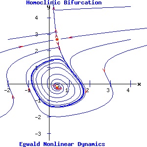
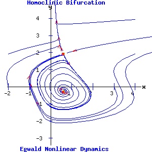
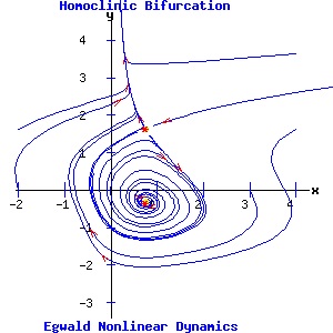
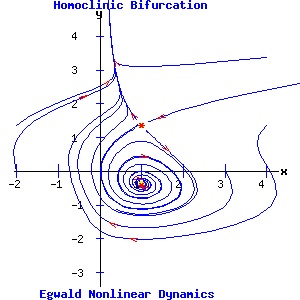
Homoclinic (Saddle-Loop, Blue Sky) Bifurcation

The saddle-node and infinite period bifurcations involve the bifurcation of limit cycles around an attractor (saddle-node) or repeller (infinite period). The saddle-loop bifurcation involves the interaction between a saddle point and a limit cycle. As a parameter varies, the unstable manifold of the saddle point feeding onto the limit cycle turns into a homoclinic orbit, and destroys the limit cycle.

In Cartesian coordinates, the system is (Medio 169-171):

d x / dt = a * y + b * x * (c - y²),         (15)

d y / dt = -x + α.         (16)

The fixed points of this system are:

(x₁, y₁) = ( α, (1/(2 * b * α)) * (a + sqrt(a² + 4 * b² * α² * c)) ),

(x₂, y₂) = ( α, (1/(2 * b * α)) * (a + sqrt(a² - 4 * b² * α² * c)) ).

The Jacobian matrix is:

The example in the diagrams below sets a = 0.7, b = 0.7, and c = .5.

The control parameter is α. Initially for α = .4, the system has a saddle point and an attracting limit cycle enclosing a repeller. As α increases, the fixed points move closer to each other, but maintain their properties. At values of α below the critical value, α_c, one unstable manifold of the saddle point feeds onto the limit cycle. At α = α_c = .75, this manifold forms a homoclinic orbit, merging with the limit cycle, and terminating at the saddle point. For α > α_c, the limit cycle is destroyed as the unstable manifold bypasses the saddle point, converging with the saddle point's other unstable manifold.

References.

• Bachratý, Viktor. Bifurcations in economic models.
• Billups, Stephen C. FINAL REPORT OF THE UCDHSC MATHEMATICS CLINIC Modeling Tissue Dynamics. University of Colorado at Denver and Health Sciences Center Mathematics Department. Spring Semester 2007.
• Boyce, William E. and Richard C. DiPrima. Elementary Differential Equations and Boundary Value Problems. New York: John Wiley, 1997.
• Burden, Richard L. and J. Douglas Faires. Numerical Analysis. 6th ed. Pacific Grove: Brooks/Cole, 1997.
• Demmel, James W. Applied Numerical Linear Algebra. Philadelphia: Siam, 1997.
• Devaney, Robert L. An Introduction to Chaotic Dynamical Systems. Menlo Park, CA: Benjamin/Cummings, 1986.
• Elaydi, Saber N. Discrete Chaos. Boca Raton: Chapman & Hall, 2000.
• Kaplan, Wilfred. Ordinary Differential Equations. Reading: Addison-Wesley, 1958.
• Lorenz, Hans-Walter. Nonlinear Dynamical Economics and Chaotic Motion. Berlin: Springer-Verlag, 1993.
• Markley, Nelson G. Principles of Differential Equatiosn. Hoboken, N.J.: John Wiley, 2004.
• Mathews, John H. and Kurtis D. Fink. Numerical Methods Using MATLAB. 3rd ed. Upper Saddle River: Prentice Hall, 1999.
• Medio, Alfredo. Chaotic Dynamics: Theory and Applications to Economics. New York: Cambridge UP, 1992.
• Nagata, K. Wayne. Nonlinear Dynamics and Chaos: Mathematics 345 Lecture Notes. Vancouver: University of B.C., 2006.
• Puu, TÖnu. Attractions, Bifurcations, and Chaos: Nonlinear Phenomena in Economics. New York: Springer, 2000.
• Strang, Gilbert. Linear Algebra and Its Applications. 3d ed. San Diego: Harcourt, 1976.
• Strogatz, Steven H. Nonlinear Dynamics and Chaos. Cambridge MA: Perseus, 1994.
• Watkins, David S. Fundamentals of Matrix Computations. New York: John Wiley, 1991.