Egwald Mathematics: Nonlinear Dynamics:

Two Dimensional Flows and Phase Diagrams

by

Elmer G. Wiens

Egwald's popular web pages are provided without cost to users.
Please show your support by joining Egwald Web Services as a Facebook Fan:

introduction | linear systems | linear stability diagram
nonlinear systems | fixed points | strogatz example | linearized stability | jacobian matrix
nonlinear stability classification | topological classifications | strogatz example | direction field
phase portrait | boyce diprima example | basin of attraction | oscillating pendulum | oscillating pendulum graphics
Lotka-Volterra-Goodwin model | predator prey phase portrait | L-V-G model with non-constant returns
references

Introduction

One can describe the dynamics of a two dimensional, continuous time process by a pair of differential equations and initial conditions:

dx / dt = f(x, y),         (1)

dy / dt = g(x, y),         (2)

  x(0) = x0,   y(0) = y0,       (3)

whose solution is a pair of functions of time, x(t) and y(t).

This process is also described using the notation:

dx₁ / dt = f₁(x₁, x₂),

dx₂ / dt = f₂(x₁, x₂),

  x₁(0) = x0₁,   x₂(0) = x0₂.

In vector notation, these dynamics are described as:

( dx₁/dt,  dx₂/dt )^T = ( f₁(x₁, x₂),  f₂(x₁, x₂) )^T,   or

x^T = (x₁, x₂),     f^T( x ) = ( f₁(x₁, x₂),  f₂(x₁, x₂) ), and

d x / dt = f( x ),

x^T(0) = (x0₁,   x0₂).

where "T" indicates the transpose from a column vector to a row vector.

Linear Systems

The simplest two dimensional, continuous time process is the second order, linear homogeneous system with constant coefficients:

dx₁ / dt = a * x₁ + b * x₂,

dx₂ / dt = c * x₁ + d * x₂

Let the matrix A be:

and the column vectors x and dx / dt be:

x^T = (x₁, x₂),

dx^T / dt = ( dx₁ / dt,   dx₂ / dt ).

The linear system has the form:

dx / dt = A * x.         (5)

The origin, o^T = (0, 0), is an equilibrium (fixed) point of (5) because A * o = o. One can examine the behaviour (stability) of the solution vector:

x^T(t) = ( x₁(t),   x₂(t) ),

near the origin, o, by analyzing the eigenvalues and eigenvectors of A.

Click to pop a new window with this analysis in detail: Classification of the Equilibrium Point at the Origin.

The general 2 by 2 matrix, A, has:

p = trace(A) = a + d, and

q = det(A) = a*d - b*c.

Its characteristic equations is:

f(µ)   =   µ² - p * µ + q

Factoring this quadratic equation yields the pair of eigenvalues, µ₁ and µ₂, where:

µ₁ = { p + sqrt(p² - 4 * q) } / 2 , and

µ₂ = { p - sqrt(p² - 4 * q) } / 2.        

Moreover:

p = µ₁ + µ₂,

q = µ₁ * µ₂.

Designate the discriminant of the characteristic equation by:

d = disc(A) = p² - 4 * q.

Classification of Fixed Points for Linear Systems

The following diagram classifies the fixed points (critical points) of the linear system (5) according to the values of p = trace(A), q = det(A), and d = disc(A). The parabola, p² - 4 * q = 0, is the locus of points (p, q) for which d = 0.

In the region of the (q, p) plain enclosed by the parabola, d = p² - 4 * q < 0. Consequently, the eigenvalues µ₁ and µ₂ are complex numbers. If p is not zero, complex eigenvalues result in spiral trajectories. If p = 0, eigenvalues are purely imaginary and trajectories enclose the fixed point in ellipses or circles.

If p > 0 and q > 0 (the positive quadrant of the (q, p) plain), both eigenvalues have positive real parts (or are purely positive numbers), and the fixed point is unstable. If p > 0, and q = 0, one eigenvalue is positive and the other is zero: the trajectories are unstable lines.

Conversely, if p < 0 and q > 0 (the negative quadrant), both eigenvalues have negative real parts (or are purely negative numbers), and the fixed point is stable. If p < 0, and q = 0, one eigenvalue is negative and the other is zero: the trajectories are stable lines.

However, if q < 0, one eigenvalue is a positive number and the other is negative: trajectories follow the saddle point pattern.

Nonlinear Systems

The general form of a two-dimensional nonlinear system is:

dx / dt = f(x, y),         (6)

dy / dt = g(x, y),         (7)

  x(t₀) = x0,   y(t₀) = y0,       (8)

Fixed Points

The fixed points of the nonlinear system are numbers x^* and y^* such that:

f(x^*, y^*) = 0, and     (9)

g(x^*, y^*) = 0,         (10)

are satisfied simultaneously. Fixed points occur where the locus of points of equations (9) and (10) intersect.

Example: (Strogatz 151-152)

The nonlinear system with functions f and g given by:

dx / dt = f(x, y) = -x + x³,

dy / dt = g(x, y) = -2 * y,

has the fixed points that satisfy:

f(x, y) = -x + x³ = 0,

g(x, y) = -2 * y = 0.

In the diagram below, the fixed points occur are the intersections of the lines x = -1, x = 0, and x = 1 with the line y = 0 (the x-axis). These four lines are called nullclines.

These fixed points are:

(x₁^*, y₁^*) = (0, 0),  

(x₂^*, y₂^*) = (-1, 0),

  (x₃^*, y₃^*) = (1, 0). 

Linearized Stability

The dynamics of a nonlinear system near a fixed point can be analyzed by linearizing the system about the fixed point, (x^*, y^*).

Jacobian Matrix

The Jacobian matrix of the nonlinear system described by the equations (6), and (7) at the fixed point (x^*, y^*) is the matrix of partial derivatives of the functions f and g evaluated at (x^*, y^*) given by:

The Jacobian matrix of constant coefficients, J, is identified with the matrix A of linear systems. Near a fixed point (x^*, y^*), the dynamics of the nonlinear system are qualitatively similar to the dynamics of the linear system associated with the J(x^*, y^*) matrix, provided the eigenvalues of the J matrix have non-zero real parts. Fixed points with a J matrix such that Re(µ_{1, 2}) ≠ 0 are called hyperbolic fixed points. Otherwise, fixed points are non-hyperbolic fixed points, whose stabilities must be determined directly.

Classification of Fixed Points for Nonlinear Systems

Let the Jacobian matrix J evaluated at a fixed point (x^*, y^*) be:

For this matrix J:

p = trace(J) = a + d, and

q = det(J) = a*d - b*c.

Its characteristic equations is:

f(µ)   =   µ² - p * µ + q

Factoring this quadratic equation yields the pair of eigenvalues, µ₁ and µ₂, where:

µ₁ = { p + sqrt(p² - 4 * q) } / 2 , and

µ₂ = { p - sqrt(p² - 4 * q) } / 2.        

Moreover:

p = µ₁ + µ₂,

q = µ₁ * µ₂.

Topological Classification

Linear stability analysis works for a hyperbolic fixed point (Re(µ_{1, 2}) ≠ 0). The nonlinear system's phase portrait near the fixed point is topologically unchanged due to small perturbations, and its dynamics are structurally stable or robust.

Linear stability analysis may fail for a non-hyperbolic fixed point: ( Re(µ_{1, 2}) = 0, or at least one µ_i = 0 ).

The classifications for the fixed points of a nonlinear system are summarized in the following diagram:

Example: (Strogatz 151-152)

The Jacobian matrix for the example is:

Stability at (x₁^*, y₁^*) = (0, 0)

For J(0, 0), p = -3, and q = 2. Thus, d = p² - 4 * q = 1; µ₁ = -1, µ₂ = -2, and (0, 0) is a hyperbolic fixed point. Consequently, the nonlinear system has a stable node (attractor) at (x₁^*, y₁^*) = (0, 0).

Stability at (x₂^*, y₂^*) = (-1, 0)

For J(-1, 0), p = 0, and q = -4. Thus, d = p² - 4 * q = 16; µ₁ = -2, µ₂ = 2, and (-1, 0) is a hyperbolic fixed point. Consequently, the nonlinear system has a saddle point at (x₂^*, y₂^*) = (-1, 0).

Stability at (x₃^*, y₃^*) = (1, 0)

Similarly, for J(1, 0), p = 0, and q = -4. Thus, d = p² - 4 * q = 16; µ₁ = -2, µ₂ = 2, and (1, 0) is a hyperbolic fixed point. Consequently, the nonlinear system has a saddle point at (x₃^*, y₃^*) = (1, 0).

Direction Field and Phase Portrait

The stability analysis for this example is verified by the following direction field and phase portrait of the nonlinear system:

The phase portrait confirms the presence of the two saddle points and fixed point attractor suggested by the direction field diagram.

Example: (Boyce and DiPrima 487-488)

The nonlinear system with functions f and g given by:

dx / dt = f(x, y) = y,                    

dy / dt = g(x, y) = -9 * sin(x) - (1/5) * y,

has the fixed points that satisfy:

f(x, y) = y = 0,                    

g(x, y) = -9 * sin(x) - (1/5) * y = 0.

The fixed points of this nonlinear system occur at the intersections of the x-nullcline, y = 0, and the y-nullcline, y = -45 * sin(x), as displayed in the next diagram.

Fixed Points

The fixed points are the points (x^*, y^*) = (n * π, 0), for n = ... -2, -1, 0, 1, 2 ....

Jacobian Matrix

The Jacobian matrix for the example is:

Stability: n = 0 or n even

If n = 0, or if n is an even number, p = -.2 < 0, q = 9 > 0: The fixed points are hyperbolic, attractors.

Stability: n odd

If n is an odd number, p = -.2 < 0, q = -9 < 0: The fixed points are hyperbolic, saddle points.

Phase Portrait

The following phase portrait of the nonlinear system verifies the stability analysis for this example.

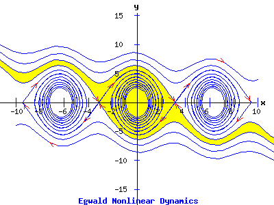
Basin of Attraction

The basin of attraction of an attracting fixed point is the set of all initial points whose solution trajectories lead to the fixed point. In the next diagram, the yellow set is the basin of attrction of the hyperbolic attractor at the origin.

Homoclinic Orbits

Solution trajectories that begin and terminate at the same fixed point, are called homoclinic orbits. An example appears in the next diagram, with the homoclinic orbits in red.

This nonlinear system has functions f and g given by:

dx / dt = f(x, y) = y,        

dy / dt = g(x, y) = x - x³,

with a saddle point at (0, 0), and centers at (-1, 0), and (1, 0).

Heteroclinic Orbits

Solution trajectories that begin and terminate at different saddle points, are called heteroclinic orbits. An example appears in the next diagram, with the heteroclinic orbits in red.

This nonlinear system has functions f and g given by:

dx / dt = f(x, y) = y,        

dy / dt = g(x, y) = -sin(x),

The fixed points are the points (x^*, y^*) = (n * π, 0), for n = ... -2, -1, 0, 1, 2 ....

If n = 0, or if n is an even number, the fixed points are centers.  If n is an odd number, the fixed points are hyperbolic, saddle points.

Physical Interpretation:
The Oscillating Pendulum (Boyce and DiPrima 476-477)

An object of mass m is suspended from a point O by a rigid, but weightless, rod of length L. The angle of the rod with the vertical is θ, with the counterclockwise direction as positive. The rod can swing or rotate about O. The gravitational force is F = m * g, while the damping force opposing the direction of motion is c * |dθ / dt|, where c is a positive constant. The tangential component of the gravitational force is F1 = -m * g * sin(θ). (See the diagram below.)

With the damping force, the equation for the angular momentum about O is:

m * L² * d²θ / dt² = - c * L * dθ/dt - m * g * L * sin(θ), or

m * L² * d²θ / dt² + c * L * dθ/dt + m * g * L * sin(θ) = 0.

Letting γ = c / (m * L), ω² = g / L, the equation of motion is:

d²θ/dt² + γ * dθ/dt + ω² * sin(θ) = 0.

This system can be converted into a two dimensional nonlinear system by letting x = θ and y = dθ/dt:

dx / dt = y, and      

dy /dt = -ω² * sin(θ) - γ * y.

Setting ω² = 9, and γ = (1/5), we get the example displayed in the phase portrait above. The relevant portion of the phase portrait is identified for x between -pi and +pi.

Oscillating Pendulum Dynamics

The next graphic displays the motion of this pendulum ( ω² = 9, and γ = (1/5) ) starting from a position slightly displaced from the vertical ( x = -3.04159 radians, y = 0.010000 radians / second ). Time is set at t = 0 seconds at this initial position. The position of the pendulum, x is given in degrees and radians from its position of rest; the angular velocity or time rate of change of x, the variable y, is measured in radians per second.

Oscillating Pendulum with Damping

Oscillating Pendulum with Damping

Lotka—Volterra—Goodwin
Predator-Prey Model (Lorenz 60-69)

The nonlinear system with functions f and g given by:

dx / dt = f(x, y) = a * x - b * x * y,

dy / dt = g(x, y) = -c * y + d * x * y,

has fixed points that satisfy:

f(x, y) = a * x - b * x * y = 0,

g(x, y) = -c * y + d * x * y = 0.

where a, b, c, d > 0 are parameters that represent the interaction between the entities of the model (x = prey population; y = predator population).

These fixed points are (x₁^*, y₁^*) = (0, 0), and (x₂^*, y₂^*) = (c / d,  a / b).

Jacobian Matrix

The Jacobian matrix is:

The trivial fixed point is a hyperbolic, saddle point, since q = det(J) = -a * c < 0.

At (x₂^*, y₂^*) = (c / d,  a / b), the Jacobian has p = trace(J) = 0, and q = det(J) = a * c > 0. Consequently, the eigenvalues are purely imaginary, nonzero, complex conjugate numbers, and the fixed point is non-hyperbolic, neutrally stable.

With a = 3, b = 2, c = 3, and d = 2, the dynamics of the following diagram reveal a center at (x₂^*, y₂^*) = (3 / 2,  3 / 2), and a saddle point at (x₁^*, y₁^*) = (0, 0):

In the Richard Goodwin version of the model, x represents the employment rate (employment relative to population), while y represents the income share of labour (the wage rate times labour employed relative to output).

In terms of the Lotka-Volterra model, the employment rate is the prey, while the wage bill is the predator.

Lotka—Volterra Model
Decreasing and Increasing Returns

The Lotka—Volterra model is sensitive to modifications in the differential equations that describe the dynamics of the nonlinear system. The following system is a perturbation in the structure of the model.

Consider the nonlinear system with functions f and g given by:

dx / dt = f(x, y) = 3 * x - 2 * x * y,               

dy / dt = g(x, y) = -3 * y + 2 * x * y - e * y * y,

where the parameter e is either between -2 and 0, or greater than 0. (The case for e = 0 appears above.) The parameter, e, measures the decreasing returns (e > 0), or increasing returns (e < 0) available to the entity represented by the variable y.

The fixed points are (x₁^*, y₁^*) = (0, 0), and (x₂^*, y₂^*) = (3/2 + (3/4)*e,   3/2). ( x₂^* > 0 requires e > -2. )

Jacobian Matrix

The Jacobian matrix is:

At (x₁^*, y₁^*) = (0, 0), p = trace(J) = 0, and q = det(J) = -9, so the trivial fixed point is a hyperbolic, saddle point.

At (x₂^*, y₂^*) = ( 3/2 + (3/4)*e,   3/2 ),   p = trace(J) = -(3/2)*e, and q = det(J) = (9/2)*e+9.   For e > 0, p < 0 and q > 0.   Consequently, (x₂^*, y₂^*) is a hyperbolic, attractor fixed point.   For -2 < e < 0, p > 0 and q > 0. Consequently, (x₂^*, y₂^*) is a hyperbolic, repeller fixed point.

References.

• Boyce, William E. and Richard C. DiPrima. Elementary Differential Equations and Boundary Value Problems. New York: John Wiley, 1997.
• Burden, Richard L. and J. Douglas Faires. Numerical Analysis. 6th ed. Pacific Grove: Brooks/Cole, 1997.
• Demmel, James W. Applied Numerical Linear Algebra. Philadelphia: Siam, 1997.
• Devaney, Robert L. An Introduction to Chaotic Dynamical Systems. Menlo Park, CA: Benjamin/Cummings, 1986.
• Elaydi, Saber N. Discrete Chaos. Boca Raton: Chapman & Hall, 2000.
• Erdi, Péter. Complexity Explained. Berlin: Springer, 2007
• Intriligator, M. D. Mathematical Optimization and Economic Theory. Englewood Cliffs: Prentice-Hall, 1971.
• Kaplan, Wilfred. Ordinary Differential Equations. Reading: Addison-Wesley, 1958.
• Lipschutz, Seymour. Linear Algebra. New York: Schaum McGraw-Hill, 1968.
• Lorenz, Hans-Walter. Nonlinear Dynamical Economics and Chaotic Motion. Berlin: Springer-Verlag, 1993.
• Mathews, John H. and Kurtis D. Fink. Numerical Methods Using MATLAB. 3rd ed. Upper Saddle River: Prentice Hall, 1999.
• Nagata, K. Wayne. Nonlinear Dynamics and Chaos: Mathematics 345 Lecture Notes. Vancouver: University of B.C., 2006
• Press, William H., Brian P. Flannery, Saul A. Teukolsky, and William T. Vetterling. Numerical Recipes: The Art of Scientific Computing. Cambridge: Cambridge UP, 1989.
• Strang, Gilbert. Linear Algebra and Its Applications. 3d ed. San Diego: Harcourt, 1976.
• Strogatz, Steven H. Nonlinear Dynamics and Chaos. Cambridge MA: Perseus, 1994.
• Wan, Henry Y. Jr. Economic Growth. New York: Harcourt, 1971.
• Watkins, David S. Fundamentals of Matrix Computations. New York: John Wiley, 1991.