| |
Operations Research - Linear Programming - Dual Simplex Algorithm
by
Elmer G. Wiens
Egwald's popular web pages are provided without cost to users.
Follow Elmer Wiens on Twitter:

Graphical Solution |
Simplex Algorithm |
Primal Simplex Tableaux Generator |
Dual Simplex Algorithm |
Dual Simplex Tableaux Generator
Economics Application - Profit Maximization |
Economics Application - Least Cost Formula
introduction | example problem | simplex algorithm | unbounded & unfeasible problems | degeneracy | references
The dual simplex method is often used in situations where the primal problem has a number of equality constraints generating artificial variables in the l.p. canonical form. Like in the primal simplex method, the standard form for the dual simplex method assumes all constraints are <=, or = constraints, but places no restrictions on the signs of the RHS bi variables.
The dual simplex algorithm consists of three phases. Phase 0 is identical to Phase 0 of the primal simplex method, as the artificial variables are replaced by the primal variables in the basis. However, the dual simplex algorithm in Phase 1 searches for a feasible dual program, while in Phase 2, it searches for the optimal dual program, simultaneously generating the optimal primal program.
Solve an example problem.
The following example will be solved using the dual simplex algorithm (Restrepo, Linear Programming, 83-90), to illustrate this technique. It is the same problem solved with the primal simplex algorithm.
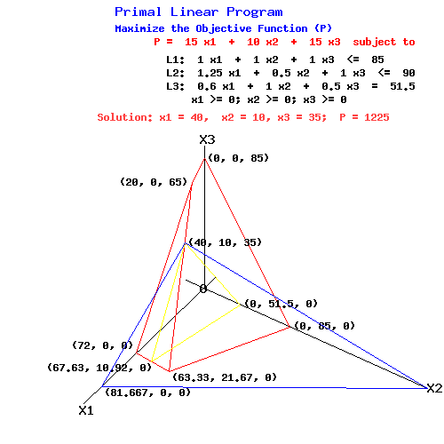
Primal Linear Program
Maximize the Objective Function (P)
P = 15 x1 + 10 x2 + 15 x3 subject to
L1: 1.0 x1 + 1.0 x2 + 1.0 x3 <= 85
L2: 1.25 x1 + 0.5 x2 + 1.0 x3 <= 90
L3: 0.6 x1 + 1.0 x2 + 0.5 x3 = 51.5
x1 >= 0; x2 >= 0; x3 >= 0
|
The following diagram illustrates the constraints and the objective function at its maximum value.
P-Plane passing through (81.667, 0, 0), (0, 122.5, 0), and (40, 10, 35) when P = 1225
L1-plane passing through (63.33, 21.67, 0), (0, 85, 0), (0, 0, 85), and (20, 0, 65)
L2-plane passing through (72, 0, 0), (63.33, 21.67, 0), and (20, 0, 65)
L3-plane passing through (67.63, 10.92, 0), (0, 51.5, 0), and (40, 10, 35)
L1-plane & L2-plane intersect along the line passing through (63.33, 21.67, 0) and (20, 0, 65)
With P = 1225, the P-plane intersects the primal feasible set only at the point (40, 10, 35).
|
If necessary, multiply any = constraints by -1 to get the RHS negative, and introduce the slack variables into the statement of the problem. The variable s3 is an artificial variable, since the third constraint is an equation.
Primal Linear Program
Maximize the Objective Function (P)
P = 15 x1 + 10 x2 + 15 x3 subject to
L1: 1.0 x1 + 1.0 x2 + 1.0 x3 + s1 = 85
L2: 1.25 x1 + 0.5 x2 + 1.0 x3 + s2 = 90
L3: -0.6 x1 - 1.0 x2 - 0.5 x3 + s3 = -51.5
x1 >= 0; x2 >= 0; x3 >= 0
s1 >= 0; s2 >= 0; s3 >= 0
|
Dual Linear Program
Minimize the Objective Function (D)
D = 85 y1 + 90 y2 - 51.5 y3 subject to
G1: 1.0 y1 + 1.25 y2 - 0.6 y3 - t1 = 15
G2: 1.0 y1 + 0.5 y2 - 1.0 y3 - t2 = 10
G3: 1.0 y1 + 1.0 y2 - 0.5 y3 - t3 = 15
y1 >= 0; y2 >= 0; y3 sign unrestriced
t1 >= 0; t2 >= 0; t3 >= 0
|
The standard forms for the primal and dual problems can be stated with the slack variables s and t:
Primal Linear Program
Maximize the Objective Function (P)
P = cT x subject to
|
|
|
Dual Linear Program
Minimize the Objective Function (D)
D = yT b subject to
|
|
|
A x + s = b, x >= 0, s >= 0
|
yT A - tT = cT, y >= 0, t >= 0
|
Dual Simplex Algorithm
The standard form for the initial dual simplex tableau is:
| Initial Tableau |
| b | A | I3 |
| 0 | -cT | O3T |
In the dual simplex algorithm, a sequence of tableaux are calculated. A given Tableauk has the form:
after consolidating the center 2 by 2 block of matrices.
|
Phase 0 - drive all artificial variables (associated with = constraints) to zero, i.e. eliminate them from the basis;
Phase I - find a tableau with Ø >= 0, i.e. a feasible dual program;
Phase II - generate tableaux that decrease the value of µ turning ß >= 0, without dropping back into Phase 0 or I, i.e. find a feasible basic dual program that minimizes the objective function D.
|
Using the initial canonical from, label rows & columns. Use the data from the example to fill in the initial tableau. Label column s3 with a * to indicate that it is an artificial variable. Add the column of row sums used to check arithmetic, and the row labelled -P / L, that will be used in Phases I and II.
| Tableau0 |
| |
b0 |
x01 |
x02 |
x03 |
s01 |
s02 |
s03* |
row
sum |
| L01 |
85 | 1.00 |
1.00 | 1.00 |
1.00 | 0.00 |
0.00 | 89 |
| L02 |
90 | 1.25 |
0.50 | 1.00 |
0.00 | 1.00 |
0.00 | 93.75 |
| L03 |
-51.5 | -0.60 |
-1.00 | -0.50 |
0.00 | 0.00 |
1.00 | -52.6 |
| P0 |
0.00 | -15 |
-10 | -15 |
0.00 | 0.00 |
0.00 | -40 |
| -P / L |
| |
| |
| |
| |
Tableau0 solution:
Variables s1, s2, s3 are the basic variables, since their columns are e1T = (1, 0, 0, 0), e2T = (0, 1, 0, 0), and e3T = (0, 0, 1, 0). The primal program is sT = (85, 90, -51.5), with xT = (0.00, 0.00, 0.00). The primal objective function has the value P = cTx = c1x1 + c2x2 + c3x3 = 0.00.
Proceed to the next tableau as follows:
Phase 0. Drive the artificial variables from the basis.
A. In Tableau0:
1. Select an artificial variable in the basis: s*3 = e3.
2. Select a nonzero element in row L3 as pivot: x3,1 = -.6.
B. To Create Tableau1:
3. Compute row L13 = L03 / (-0.6).
4. Subtract multiples of row L13 from all other rows of Tableau0 so that x11 = e3 in Tableau1.
| Tableau1 |
| |
b1 |
x11 |
x12 |
x13 |
s11 |
s12 |
s13* |
row
sum |
| L11 = L01 - 1.0 L13 |
-0.8333 | 0.00 |
-0.6667 | 0.1667 |
1.00 | 0.00 |
1.667 | 1.3334 |
| L12 = L02 - 1.25 L13 |
-17.292 | 0.00 |
-1.5834 | -0.0417 |
0.00 | 1.00 |
2.0834 | -15.8333 |
| L13 = L03 / (-0.6) |
85.8333 | 1.00 |
1.6667 | 0.8333 |
0.00 | 0.00 |
-1.6667 | 87.6667 |
| P1 = P0 - (-15) L13 |
1287.5 | 0.00 |
15 | -2.5 |
0.00 | 0.00 |
-25 | 1275 |
| -P1 / L11 |
| |
22.5 | 15 |
| |
| |
Tableau1 solution:
Basis: x1, s1, s2.
The primal unfeasible program: xT = (85.8333, 0.00, 0.00); sT = (-0.8333, -17.292, 0).
The primal objective function has the value P = 1287.5.
Proceed to the next tableau as follows: Since the artificial variable s*3 associated with the = constraint is not in the basis, Phase 0 is complete.
Phase I. Obtain nonnegative entries in Ø (the second last row) for the sign-restricted primal and slack variables. Since Ø13 = -2.5 is negative, the algorithm is in Phase I.
Goal: Generate a feasible dual program so that Ø >= 0.
A. In Tableau1:
1. Select a target column, col, with Øcol < 0: Ø13 = -2.5, col = 3.
2. Select any row, r, with a positive entry in col 3 as the pivot row: row = 1 associated with constraint L1: x1,3 = 0.1667.
3. Compute the ratios -Ø / L1 as per the last row. Discard ratios which are not positive and ratios associated with artificial variables.
Select the column with the least positive ratio as the pivot column: 15 in col = 3. Thus x1,3 = 0.1667 is the pivot; slack variable s1 will leave the basis; x3 will enter the basis.
B. To Create Tableau2:
4. Compute row L21 = L11 / (0.1667).
5. Subtract multiples of row L21 from all other rows of Tableau1 so that x23 = e1 in Tableau2.
| Tableau2 |
| |
b2 |
x21 |
x22 |
x23 |
s21 |
s22 |
s23* |
row
sum |
| L21 = L11 / ( 0.1667) |
-5.00 | 0.00 |
-4.00 | 1.00 |
6.00 | 0.00 |
10.00 | 8.00 |
| L22 = L12 - (-0.0417 ) L21 |
-17.50 | 0.00 |
-1.75 | 0.00 |
0.25 | 1.00 |
2.5 | -15.5 |
| L23 = L13 - 0.8333 L21 |
90.00 | 1.00 |
5.00 | 0.00 |
-5.00 | 0.00 |
-10.00 | 81 |
| -P2 = P1 - (-2.5000 ) L21 |
1275 | 0.00 |
5.00 | 0.00 |
15.00 | 0.00 |
0.00 | 1295 |
| P2 / L22 |
| |
2.8571 | |
| |
| |
Tableau2 solution:
Basis: x1, x2, s2.
The primal unfeasible program: xT = (83.75, 1.25, 0.00); sT = (0, -15.313, 0).
The primal objective function has the value P = 1275.
Proceed to the next tableau as follows: Since Ø2 >= 0. The algorithm is in Phase II.
Phase II. Goal: Generate an optimal program so that ß >= 0.
A. In Tableau2:
1. Select a target row, r, with br < 0: b22 = -17.5, r = 2.
2. Compute the ratios -Ø / L2 as per the last row. Discard ratios which are not positive, and ratios associated with artificial variables.
Select the column with the least positive ratio as the pivot column: 2.8571 in col = 2. Thus x2,2 = -1.75 is the pivot; slack variable s2 will leave the basis; x2 will enter the basis.
B. To Create Tableau3:
3. Compute row L32 = L22 / (-1.75).
4. Subtract multiples of row L32 from all other rows of Tableau2 so that x32 = e2 in Tableau3.
| Tableau3 |
| |
b3 |
x31 |
x32 |
x33 |
s31 |
s32 |
s33* |
row
sum |
| L31 = L21 - (-4.00) L32 |
35 | 0.00 |
0.00 | 1.00 |
5.4286 | -2.2857 |
4.2857 | 43.4286 |
| L32 = L22 / (-1.75) |
10.00 | 0.00 |
1.00 | 0.00 |
-0.1429 | -0.5714 |
-1.4286 | 8.8571 |
| L33 = L23 - 5.00 L32 |
40.00 | 1.00 |
0.00 | 0.00 |
-4.2857 | 2.8571 |
-2.8571 | 36.7143 |
| P3 = P2 - 5.00 L32 |
1225 | 0.00 |
0.00 | 0.00 |
15.7143 | 2.8571 |
7.1429 | 1250.7143 |
| -P / L |
| |
| |
| |
| |
Tableau3 solution:
Basis: x1, x2, x3.
The primal feasible program: xT = (40, 10, 35); sT = (0, 0, 0).
The primal objective function has the value P = 1225.
For this tableau, b >= 0, the artificial variable, s*3, is not in the basis, and all entries in the last row corresponding to the variables x1, x2, x3, s1, and s2 are nonnegative.
The dual simplex algorithm terminates, since all conditions of Phase I and II are satisfied.
The optimal programs are:
x = (40, 10, 35), s = (0, 0, 0); y = (15.71, 2.86, 7.14), t = (0, 0, 0); P = 1225.
Unbounded and Unfeasible Problems.
As shown on the graphical web page, and on the simplex algorithm web page,
the next example has an unbounded primal solution, with an unfeasible dual problem.
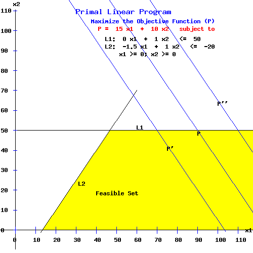
Primal Linear Program
Maximize the Objective Function (P)
P = 15 x1 + 10 x2 subject to
L1: 0 x1 + 1.0 x2 <= 50
L2: -1.5 x1 + 1.0 x2 <= -20
x1 >= 0; x2 >= 0
|
Dual Linear Program
Minimize the Objective Function (D)
D = 50 y1 - 20 y2 subject to
G1: 0 y1 - 1.5 y2 >= 15
G2: 1.0 y1 + 1.0 y2 >= 10
y1 >= 0; y2 >= 0
|
To solve this problem using the dual simplex algorithm, set up the initial tableau as usual:
| Tableau0 |
| |
b0 |
x01 |
x02 |
s01 |
s02 |
row
sum |
| L01 |
50 | 0.00 |
1.00 | 1.00 |
0.00 | 52 |
| L02 |
-20 | -1.5 |
1.00 | 0.00 |
1.00 | -19.5 |
| P0 |
0.00 | -15 |
-10 | 0.00 |
0.00 | -25 |
| -P / L |
| |
10 | |
| |
Phase 0: Complete since there are no artificial variables.
Phase I: Since Ø01 = -15 and Ø02 = -10 are negative, the algorithm is in Phase I.
Goal: Generate a feasible program so that Ø >= 0.
A. In Tableau0:
1. Select a target column, col, with Øcol < 0: Ø12 = -10, col = 2.
2. Select any row, r, with a positive entry in col 2 as the pivot row: row = 1 associated with constraint L1: x1,2 = 1.00. (Note: must select target col = 2 for this to work)
3. Compute the ratios -Ø / L1 as per the last row. Discard ratios which are not positive and ratios associated with artificial variables. Select the column with the least positive ratio as the pivot column: 10 in col = 2. Thus x1,2 = 1.00 is the pivot; slack variable s1 will leave the basis; x2 will enter the basis.
B. To Create Tableau1:
4. Compute row L11 = L10 / (1.00).
5. Subtract multiples of row L11 from all other rows of Tableau0 so that x12 = e1 in Tableau1.
| Tableau1 |
| |
b1 |
x11 |
x12 |
s11 |
s12 |
row
sum |
| L11 = L01 / 1 |
50 | 0.00 |
1.00 | 1.00 |
0.00 | 52 |
| L12 = L02 - 1 L11 |
-70.00 | -1.50 |
0.00 | -1.00 |
1.00 | -71.50 |
| P1 = P0 - (-15) L11 |
500 | -15.00 |
0.00 | 10.00 |
0.00 | 495 |
| -P / L |
| |
| |
| |
Phase I: Since Ø11 = -15 is negative, the algorithm is in Phase I. However, no positive entry exists in the target column = 1, so no pivot exists. The algorithm breaks down. The dual program is unfeasible.
As the following diagram shows, the primal objective function P is unbounded since it intersects the feasible set for any large positive number = P.
Degeneracy and Cycling.
The primal simplex algorithm breaks down in degenerate situations in the primal l.p. problem. Since the dual simplex algorithm works on the dual l.p. problem, primal degeneracy will not affect its execution. To see this,
click to pop a new window where this
primal degenerate problem is solved with the dual simplex method.
Linear Programming References.
- Budnick, Frank S., Richard Mojena, and Thomas E. Vollmann. Principles of Operations Research for Management. Homewood: Irwin, 1977.
- Dantzig, G., A. Orden, and P. Wolfe. "The Generalized Simplex Method for Minimizing a Linear Form under Inequality Restraints." Pacific Journal of Mathematics. 8, (1955): 183-195.
-
Dantzig, George B. Linear Programming and Extensions. Princeton: Princeton U P, 1963.
-
Dorfman, R., P. Samuelson, and R. Solow. Linear Programming and Economics Analysis. New York: McGraw-Hill, 1958.
-
Hadley, G. Linear Algebra. Reading, Mass.: Addison-Wesley, 1961.
-
Hadley, G. Linear Programming. Reading, Mass.: Addison-Wesley, 1962.
- Hillier, Frederick S. and Gerald J. Lieberman. Operations Research.. 2nd ed. San Francisco: Holden-Day, 1974.
-
Karlin, S. Mathematical Methods in the Theory of Games and Programming. Vols. I & II. Reading, Mass.: Addison-Wesley, 1959.
- Loomba, N. Paul. Linear Programming: An Introductory Analysis. New York: McGraw-Hill, 1964.
- Press, William H., Brian P. Flannery, Saul A. Teukolsky, and William T. Vetterling. Numerical Recipes: The Art of Scientific Computing. Cambridge: Cambridge UP, 1989.
-
Saaty, Thomas L. Mathematical Methods of Operations Research. New York: McGraw-Hill, 1959.
- Sierksma, Gerard. Linear and Integer Programming: Theory and Practice. 2nd ed. New York: Marcel Dekker, 2002.
-
Sposito, Vincent. Linear and Nonlinear Programming. Ames, Iowa: Iowa UP, 1975.
-
Sposito, Vincent. Linear Programming with Statistical Applications. Ames, Iowa: Iowa UP, 1989.
-
Strang, Gilbert. Linear Algebra and Its Applications.3rd ed. San Diego: Harcourt, 1988.
-
Restrepo, Rodrigo A. Theory of Games and Programming: Mathematics Lecture Notes. Vancouver: University of B.C., 1967.
-
Restrepo, Rodrigo A. Linear Programming and Complementarity. Vancouver: University of B.C., 1994.
-
Taha, Hamdy A. Operations Research: An Introduction. 2nd ed. New York: MacMillan, 1976.
- Wagner, Harvey M. Principles of Management Science: With Applications to Executive Decisions. 2nd ed. Englewood Cliffs: Prentice-Hall, 1975.
- Wagner, Harvey M. Principles of Operations Research: With Applications to Managerial Decisions. 2nd ed. Englewood Cliffs: Prentice-Hall, 1975.
- Wu, Nesa, and Richard Coppins. Linear Programming and Extensions. New York: McGraw-Hill, 1981.
|
|