| |
Operations Research - Linear Programming - Simplex Algorithm
by
Elmer G. Wiens
Egwald's popular web pages are provided without cost to users.
Follow Elmer Wiens on Twitter:

Graphical Solution |
Simplex Algorithm |
Primal Simplex Tableaux Generator |
Dual Simplex Algorithm |
Dual Simplex Tableaux Generator
Economics Application - Profit Maximization |
Economics Application - Least Cost Formula
example problem | l.p. standard form | basic simplex algorithm | algorithm validity
primal simplex algorithm | unbounded & unfeasible problems | degeneracy | references
Solve an example problem.
Consider the following linear programming problem:
Primal Linear Program
Maximize the Objective Function (P)
P = 15 x1 + 10 x2 subject to
L1: 0.25 x1 + 1.0 x2 <= 65
L2: 1.25 x1 + 0.5 x2 <= 90
L3: 1.0 x1 + 1.0 x2 <= 85
x1 >= 0; x2 >= 0
|
Dual Linear Program
Minimize the Objective Function (D)
D = 65 y1 + 90 y2 + 85 y3 subject to
G1: 0.25 y1 + 1.25 y2 + 1.0 y3 >= 15
G2: 1.0 y1 + 0.5 y2 + 1.0 y3 >= 10
y1 >= 0; y2 >= 0; y3= 0
|
This problem is solved on the graphical solution web page. The primal optimal program is x = (x1, x2) = (63.333, 21.667) yielding a value for the objective function P = 1166.67. The dual optimal program is y = (y1, y2, y3) = (0, 6.67, 6.67), with an optimal value for the objective function D = 1166.67.
The Simplex L.P. Standard Form.
The above example can be stated as a particular set of data of the general canonical form.
|
A =
|
| a11 a12 |
| a21 a22 |
| a31 a32 |
|
=
|
| 0.25 1.00 |
| 1.25 0.50 |
| 1.00 1.00 |
|
I3 |
=
|
| 1.00 0.00 0.00 |
| 0.00 1.00 0.00 |
| 0.00 0.00 1.00 |
|
O3 | = | | 0 |
| 0 |
| 0 | |
| b = | | b1 |
| b2 |
| b3 | |
= | | 65 |
| 90 |
| 85 | |
c = | | c1 |
| c2 | |
= | | 15 |
| 10 | |
| x = | | x1 |
| x2 | |
s = | | s1 |
| s2 |
| s3 | |
y = | | y1 |
| y2 |
| y3 | |
t = | | t1 |
| t2 | |
The standard forms for the primal and dual problems can be stated with the slack variables s and t:
Primal Linear Program
Maximize the Objective Function (P)
P = cT x subject to
|
|
|
Dual Linear Program
Minimize the Objective Function (D)
D = yT b subject to
|
|
|
A x + s = b, x >= 0, s >= 0
|
yT A - tT = cT, y >= 0, t >= 0
|
This example l.p. problem has the nice feature that all constraints are <= constraints, and the vector of RHS coefficients b >= 0.
The Basic Simplex Algorithm.
The algorithms used on this web page are based on the lecture notes of Rodrigo A. Restrepo.
The first version of the simplex algorithm exploits the special structure of the example l.p. problem. The standard form (augemented form of the simplex algorithm for the initial simplex tableau in the basic simplex algorithm is:
| Initial Tableau |
| b | A | I3 | O3 |
| 0 | -cT | O3T | 1 |
Label rows & columns. Use the data from the example to fill in the initial tableau. Add two new columns: the column of row sums used to check arithmetic, and the column labelled b0 / x01 whose values are determined in step A. 2. below. (If you perform the simplex row operations on the column of row sums, and then check that each entry equals the sum of that row, you have a check on your arithmetic as you proceed with hand calculations.)
| Simplex Tableau0 |
| |
b0 | x01 |
x02 | s01 |
s02 | s03 |
e4 | row
sum |
b0 / x01 |
| L01 |
65 | 0.25 |
1.00 | 1.00 |
0.00 | 0.00 |
0.00 | 67.25 |
65 / .25 = 260.00 |
| L02 |
90 | 1.25 |
0.50 | 0.00 |
1.00 | 0.00 |
0.00 | 92.75 |
90 / 1.25 = 72.00 |
| L03 |
85 | 1.00 |
1.00 | 0.00 |
0.00 | 1.00 |
0.00 | 88.00 |
85 / 1.00 = 85.00 |
| P0 |
0.00 | -15 |
-10 | 0.00 |
0.00 | 0.00 |
1.00 | -24 |
|
Tableau0 solution:
Variables s1, s2, s3 are the basic variables, since their columns are e1T = (1, 0, 0, 0), e2T = (0, 1, 0, 0), and e3T = (0, 0, 1, 0). The primal program is sT = (65, 90, 85), with xT = (0.00, 0.00). The primal objective function has the value P = cTx = c1x1 + c2x2 = 0.00. The infeasible dual program (found in the bottom row) is tT = (-15, -10), and yT = (0.00, 0.00, 0.00).
Proceed to the next tableau as follows:
A. In Tableau0:
1. Since the coefficient of x1 in the last row, -15, is the most negative, x1 will enter the basis.
2. Compute the ratios bi / xi,1 as per the last column: select the row with the smallest positive ratio, L2 = 72. Thus x2,1 = 1.25 is the pivot , and slack variable s2 will leave the basis.
B. To create Tableau1:
3. Compute row L12 by dividing row L02 by the pivot = 1.25.
4. Subtract multiples of row L12 from all other rows of Tableau0 so that x11 = e2 in Tableau1.
Notes:
1. Step A.2 ensures that b1 >= 0 after step B.4.
2. Step A.1 ensures that step B.4 adds a positive number to P0: 1080 = 15*72 = 15 * (90 / 1.25) = c1 * b02 / x02,1
3. The vector x01 = .25 s01 + 1.25 s02 + 1.0 s03 - 15 e4. Since the coefficient of s02, 1.25, is not zero, x01 can replace s02 in the basis. Furthermore, the row operations of Step 3. and 4. do not change the status of vectors x01, s01,s03, and e4 as a basis of the Euclidean space E4.
| Simplex Tableau1 |
| |
b1 | x11 |
x12 | s11 |
s12 | s13 |
e4 | row
sum |
b1 / x12 |
| L11 = L01 - .25 L12 |
47 | 0.00 |
0.90 | 1.00 |
-0.20 | 0.00 |
0.00 | 48.7 |
47 / 0.9 = 52.222 |
| L12 = L02 / 1.25 |
72 | 1.00 |
0.40 | 0.00 |
0.80 | 0.00 |
0.00 | 74.2 |
72 / 0.4 = 180.00 |
| L13 = L03 - 1.0 L12 |
13 | 0.00 |
0.60 | 0.00 |
-0.80 | 1.00 |
0.00 | 13.80 |
13 / 0.6 = 21.667 |
| P1 = P0 - (-15.0) L12 |
1080.00 | 0.00 |
-4 | 0.00 |
12 | 0.00 |
1.00 | 1089 |
|
Tableau1 solution:
Variables x1, s1, s3 are basic variables. The primal program is sT = (47, 0, 13), with xT = (72., 0.00). The primal objective function has the value P = cTx = c1x1 + c2x2 = 15*72 + 4*0 = 1080.00. The infeasible dual program (found in the bottom row) is tT = (0, -4), and yT = (0.00, 12.00, 0.00).
Proceed to the next tableau as follows:
A. In Tableau1:
1. Since the coefficient of x2 in the last row, -4, is the most negative, x2 will enter the basis.
2. Compute the ratios bi / xi,2 as per the last column: select the row with the smallest positive ratio, L3 = 21.667. Thus x3,2 = 0.60 is the pivot , and slack variable s3 will leave the basis.
B. To create Tableau2:
3. Compute row L23 by dividing row L13 by the pivot = 0.60.
4. Subtract multiples of row L23 from all other rows of Tableau1 so that x22 = e3 in Tableau2.
| Simplex Tableau2 |
| |
b2 | x21 |
x22 | s21 |
s22 | s23 |
e4 | row
sum |
|
| L21 = L11 - 0.90 L23 |
27.5 | 0.00 |
0.00 | 1.00 |
1.00 | -1.50 |
0.00 | 28.0 |
|
| L22 = L12 - 0.40 L23 |
63.333 | 1.00 |
0.00 | 0.00 |
1.333 | -0.667 |
0.00 | 65.0 |
|
| L23 = L13 / 0.60 |
21.667 | 0.00 |
1.00 | 0.00 |
-1.333 | 1.667 |
0.00 | 23.0 |
|
| P2 = P1 - (-4.0) L23 |
1166.67 | 0.00 |
0.00 | 0.00 |
6.667 | 6.667 |
1.00 | 1181 |
|
Tableau2 solution:
Variables x1, x2, s1 are basic variables. The feasible primal program is sT = (27.5, 0, 0), with xT = (63.333, 21.667). The primal objective function has the value P = cTx = c1x1 + c2x2 = 15*63.333 + 4*21.667 = 1111.67. The feasible dual program (found in the bottom row) is tT = (0, 0), and yT = (0.00, 6.667, 6.667).
Since these feasible programs satisfy the complementary slackness conditions:
tTx = t1x1 + t2x2= 0
yTs = y1s1 + y2s2 + y3s3 = 0,
they are optimal programs.
Notes:
1.0 In the Final Tableau, all the coefficients in the last row corresponding to the primal variables, x1 and x2, and the slack variables are nonnegative. Therefore, the simplex algorithm terminates displaying the optimal primal and dual programs along with the optimal value of the objective function.
2.0 Each Tableau contains the unit vectors e1, e2, e3, and e4 among its columns.
3.0 A given Tableauk has the form:
4.0 The row operations performed on the matrix of each tableau are equivalent to premultiplying the tableau's matrix by some nonsingular matrix. Therefore, a nonsingular matrix B exists such that:
Tableau2 = B Tableau0
Validity of the Simplex Algorithm.
In block matrix form, the last equation is:
where B is a 4 by 4 (in the example above) nonsingular matrix, i.e. B has an inverse. The last 2 by 2 block of matrices in this equation implies:
Substituting for B in the first matrix equation, the first 2 by 2 block of matrices implies that:
Equating matrices yields:
|
1. ß = Bb,
2. U = BA,
3. µ = yTb,
4. tT = yTA - cT >= 0
|
Furthermore, since Tableau2 is the final tableau, y >= 0, so (y, t) is a feasible program for the dual problem.
By construction of Tableau0, and since row operations preserve equations in subsequent tableaus:
Ux + Bs = ß --> BAx + Bs = Bb
using 1. and 2. above. But B nonsingular implies the matrix B is nonsingular. Premultiplying by B's inverse yields:
Ax + s = b
Therefore, (x, s) is a feasible program for the primal problem.
Finally, the steps of the simplex algorithm rule that when a slack variable, sk, is in the basis, the corresponding dual variable yk = 0. If sk is not in the basis, then sk = 0. Therefore, complementary slackness obtains:
yTs = 0.
Similarly, if a primal variable, xk enters the basis (is not 0), then tk = 0. Therefore, complementary slackness obtains:
tTx = 0.
The pairs (x, s) and (y, t) are feasible and obey complementary slackness. Consequently, (x, s) is an optimal program for the primal problem, and (y, s) is an optimal program for the dual problem.
Example Block Matrices.
Look at Tableau2, and note that the basic variables, s1, x1, x2, plus the last column are the unit vectors e1, e2, e3, e4. Listing the columns corresponding to these variables in Tableau0 yields a matrix, call it AB:
| AB | = |
| s01 |
x01 |
x02 |
e4 |
| 1.00 |
0.25 |
1.00 |
0.00 |
| 0.00 |
1.25 |
0.50 |
0.00 |
| 0.00 |
1.00 |
1.00 |
0.00 |
| 0.00 |
-15 |
-10 |
1.00 |
|
Computing the inverse of AB yields a matrix found in Tableau2, namely B:
| AB-1 | = |
| s21 |
s22 |
s23 |
e4 |
| 1.00 |
1.0 |
-1.50 |
0.00 |
| 0.00 |
1.333 |
-0.6667 |
0.00 |
| 0.00 |
-1.333 |
1.6667 |
0.00 |
| 0.00 |
6.667 |
6.667 |
1.00 |
|
=
| B |
Premultiplying Tableau0 by B yields Tableau2.
The Primal Simplex Algorithm.
The basic simplex algorithm described above can be extended to handle a variety of complications, including = constraints with artificial variables, (Hadley, 108-148). However, an algorithm developed by Dantzig et al. for implementation on computers handles these complications in a straightforward manner that is amenable to hand calculation. The standard form for the primal simplex method assumes all constraints are <=, or = constraints, but places no restrictions on the signs of the RHS bi variables.
In the primal simplex algorithm, a sequence of tableaux are calculated. A given Tableauk has the form:
after consolidating the center 2 by 2 block of matrices.
This primal simplex algorithm uses a "three-phase method":
|
Phase 0 - drive all artificial variables (associated with = constraints) to zero, i.e. eliminate them from the basis;
Phase I - find a tableau with ß >= 0, i.e. a feasible primal program;
Phase II - generate tableaux that increase the value of µ, without dropping back into Phase 0 or I, until Ø >= 0 for all sign restricted variables, i.e. find a feasible primal program that maximizes the objective function.
|
The following example will be solved using the primal simplex algorithm (Restrepo, Linear Programming, 58-66), to illustrate this technique.
Primal Linear Program
Maximize the Objective Function (P)
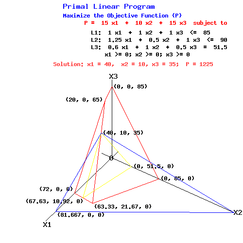
P = 15 x1 + 10 x2 + 15 x3 subject to
L1: 1.0 x1 + 1.0 x2 + 1.0 x3 <= 85
L2: 1.25 x1 + 0.5 x2 + 1.0 x3 <= 90
L3: 0.6 x1 + 1.0 x2 + 0.5 x3 = 51.5
x1 >= 0; x2 >= 0; x3 >= 0
|
Click to pop a new window with the primal and dual
l.p. problem displayed with the = constraint replaced with <= and >= constraints, and the solution obtained with the online l.p. solver.
The following diagram illustrates the constraints and the objective function at its maximum value.
P-Plane passing through (81.667, 0, 0), (0, 122.5, 0), and (40, 10, 35) when P = 1225
L1-plane passing through (63.33, 21.67, 0), (0, 85, 0), (0, 0, 85), and (20, 0, 65)
L2-plane passing through (72, 0, 0), (63.33, 21.67, 0), and (20, 0, 65)
L3-plane passing through (67.63, 10.92, 0), (0, 51.5, 0), and (40, 10, 35)
L1-plane & L2-plane intersect along the line passing through (63.33, 21.67, 0) and (20, 0, 65)
With P = 1225, the P-plane intersects the primal feasible set only at the point (40, 10, 35).
|
If necessary, multiply any = constraints by -1 to get the RHS negative, and introduce the slack variables into the statement of the problem. The variable s3 is an artificial variable, since the third constraint is an equation.
Primal Linear Program
Maximize the Objective Function (P)
P = 15 x1 + 10 x2 + 15 x3 subject to
L1: 1.0 x1 + 1.0 x2 + 1.0 x3 + s1 = 85
L2: 1.25 x1 + 0.5 x2 + 1.0 x3 + s2 = 90
L3: -0.6 x1 - 1.0 x2 - 0.5 x3 + s3 = -51.5
x1 >= 0; x2 >= 0; x3 >= 0
s1 >= 0; s2 >= 0; s3 >= 0
|
Dual Linear Program
Minimize the Objective Function (D)
D = 85 y1 + 90 y2 - 51.5 y3 subject to
G1: 1.0 y1 + 1.25 y2 - 0.6 y3 - t1 = 15
G2: 1.0 y1 + 0.5 y2 - 1.0 y3 - t2 = 10
G3: 1.0 y1 + 1.0 y2 - 0.5 y3 - t3 = 15
y1 >= 0; y2 >= 0; y3 sign unrestriced
t1 >= 0; t2 >= 0; t3 >= 0
|
The standard form for the initial primal simplex tableau is:
| Initial Tableau |
| b | A | I3 | O3 |
| 0 | -cT | O3T | 1 |
Label rows & columns. Use the data from the example to fill in the initial tableau. Label column s3 with a * to indicate that it is an artificial variable. Add two new columns: the column of row sums used to check arithmetic, and the column labelled b / xk, that will be used in Phases I and II.
| Tableau0 |
| |
b0 |
x01 |
x02 |
x03 |
s01 |
s02 |
s03* |
e4 |
row
sum |
b / xk |
| L01 |
85 | 1.00 |
1.00 | 1.00 |
1.00 | 0.00 |
0.00 | 0.00 |
89 | |
| L02 |
90 | 1.25 |
0.50 | 1.00 |
0.00 | 1.00 |
0.00 | 0.00 |
93.75 | |
| L03 |
-51.5 | -0.60 |
-1.00 | -0.50 |
0.00 | 0.00 |
1.00 | 0.00 |
-52.6 | |
| P0 |
0.00 | -15 |
-10 | -15 |
0.00 | 0.00 |
0.00 | 1.00 |
-39 | |
Tableau0 solution:
Variables s1, s2, s3 are the basic variables, since their columns are e1T = (1, 0, 0, 0), e2T = (0, 1, 0, 0), and e3T = (0, 0, 1, 0). The primal program is sT = (85, 90, -51.5), with xT = (0.00, 0.00, 0.00). The primal objective function has the value P = cTx = c1x1 + c2x2 + c3x3 = 0.00.
Proceed to the next tableau as follows:
Phase 0. Drive the artificial variables from the basis.
A. In Tableau0:
1. Select an artificial variable in the basis: s*3 = e3.
2. Select a nonzero element in row L3 as pivot: x3,1 = -.6. (I repeat the simplex algorithm with x3,2 = -1 as the pivot below.)
B. To Create Tableau1:
3. Compute row L13 = L03 / (-0.6).
4. Subtract multiples of row L13 from all other rows of Tableau0 so that x11 = e3 in Tableau1.
| Tableau1 |
| |
b1 |
x11 |
x12 |
x13 |
s11 |
s12 |
s13* |
e4 |
row
sum |
b1 / x12 |
| L11 = L01 - 1.0 L13 |
-0.8333 | 0.00 |
-0.6667 | 0.1667 |
1.00 | 0.00 |
1.667 | 0.00 |
1.3334 | 1.25 |
| L12 = L02 - 1.25 L13 |
-17.292 | 0.00 |
-1.5834 | -0.0416 |
0.00 | 1.00 |
2.0834 | 0.00 |
-15.8333 | 10.9 |
| L13 = L03 / (-0.6) |
85.8333 | 1.00 |
1.6667 | 0.8333 |
0.00 | 0.00 |
-1.6667 | 0.00 |
87.6667 | 51.49 |
| P1 = P0 - (-15) L13 |
1287.5 | 0.00 |
15 | -2.5 |
0.00 | 0.00 |
-25 | 1.00 |
1276 | |
Tableau1 solution:
Basis: x1, s1, s2.
The primal unfeasible program: xT = (85.8333, 0.00, 0.00); sT = (-0.8333, -17.292, 0).
The primal objective function has the value P = 1287.5.
Proceed to the next tableau as follows: Since the artificial variable s*3 associated with the = constraint is not in the basis, Phase 0 is complete.
Phase I. Since b11 and b12 are negative, the algorithm is in Phase I.
Goal: Generate a feasible program so that b >= 0.
A. In Tableau1:
1. Select a target row, r, with br < 0: b12 = -17.292, r = 2.
2. Select any column, col, with a negative entry in row 2 as the pivot column: col = 2 associated with variable x2, x2,2 = -1.5834.
3. Compute the ratios bi / xi,2 as per the last column.
Select the row with the smallest positive ratio: L1 = 1.25. Thus x1,2 = -0.6667 is the pivot; slack variable s1 will leave the basis; x2 will enter the basis.
To Create Tableau2:
4. Compute row L21 = L11 / (-0.6667).
5. Subtract multiples of row L21 from all other rows of Tableau1 so that x22 = e1 in Tableau2.
| Tableau2 |
| |
b2 |
x21 |
x22 |
x23 |
s21 |
s22 |
s23* |
e4 |
row
sum |
b2 / x23 |
| L21 = L11 / (- 0.6667) |
1.25 | 0.00 |
1.00 | -.25 |
-1.5 | 0.00 |
-2.5 | 0.00 |
-2 | -5 |
| L22 = L12 - (-0.15834) L21 |
-15.313 | 0.00 |
0.00 | -0.4375 |
-2.375 | 1.00 |
-1.875 | 0.00 |
-19 | 35 |
| L23 = L13 - 1.6667 L21 |
83.75 | 1.00 |
0.00 | 1.25 |
2.5 | 0.00 |
2.5 | 0.00 |
91 | 67 |
| P2 = P1 - 15 L21 |
1268.75 | 0.00 |
0.00 | 1.25 |
22.5 | 0.00 |
12.5 | 1.00 |
1306 | |
Tableau2 solution:
Basis: x1, x2, s2.
The primal unfeasible program: xT = (83.75, 1.25, 0.00); sT = (0, -15.313, 0).
The primal objective function has the value P = 1268.75.
Proceed to the next tableau as follows:
Phase I. Since b22 is negative, the algorithm is in Phase I.
Goal: Generate a feasible program so that b >= 0.
A. In Tableau2:
1. Select a target row, r, with br < 0: b22 = -15.313, r = 2.
2. Select any column, col, with a negative entry in row 2 as the pivot column: col = 3 associated with variable x3, x2,3 = -0.4375.
3. Compute the ratios bi / xi,3 as per the last column.
Select the row with the smallest positive ratio: L2 = 35. Thus x2,3 = -0.4375 is the pivot; slack variable s2 will leave the basis; x3 will enter the basis.
To Create Tableau3:
4. Compute row L32 = L22 / (-0.4375).
5. Subtract multiples of row L32 from all other rows of Tableau2 so that x33 = e2 in Tableau3.
| Tableau3 |
| |
b3 |
x31 |
x32 |
x33 |
s31 |
s32 |
s33* |
e4 |
row
sum |
|
| L31 = L21 - 0.25 L32 |
10 | 0.00 |
1.00 | 0.00 |
-0.1429 | -0.5714 |
-1.4286 | 0.00 |
8.857 | |
| L32 = L22 / (-0.4375) |
35 | 0.00 |
0.00 | 1.00 |
5.4286 | -2.2857 |
4.2857 | 0.00 |
43.43 | |
| L33 = L23 - 1.25 L32 |
40 | 1.00 |
0.00 | 0.00 |
-4.2857 | 2.8571 |
-2.8571 | 0.00 |
36.71 | |
| P3 = P2 - 1.25 L32 |
1225 | 0.00 |
0.00 | 0.00 |
15.7143 | 2.8571 |
7.1429 | 1.00 |
1251.71 | |
Tableau3 solution:
Basis: x1, x2, x3.
The primal feasible program: xT = (40, 10, 35); sT = (0, 0, 0).
The primal objective function has the value P = 1225.
For this tableau, b >= 0, the artificial variable, s*3, is not in the basis, and all entries in the last row corresponding to the variables x1, x2, x3, s1, and s2 are nonnegative.
The primal simplex algorithm terminates without proceeding to Phase II, since all conditions of Phase I and II are satisfied.
The optimal programs are:
x = (40, 10, 35), s = (0, 0, 0); y = (15.71, 2.86, 7.14), t = (0, 0, 0); P = 1225.
To demonstrate Phase II of the primal simplex algorithm, begin with Tableau0 above, but use x3,2 = -1 as the pivot.
| Tableau0 |
| |
b0 |
x01 |
x02 |
x03 |
s01 |
s02 |
s03* |
e4 |
row
sum |
b / xk |
| L01 |
85 | 1.00 |
1.00 | 1.00 |
1.00 | 0.00 |
0.00 | 0.00 |
89 | |
| L02 |
90 | 1.25 |
0.50 | 1.00 |
0.00 | 1.00 |
0.00 | 0.00 |
93.75 | |
| L03 |
-51.5 | -0.60 |
-1.00 | -0.50 |
0.00 | 0.00 |
1.00 | 0.00 |
-52.6 | |
| P0 |
0.00 | -15 |
-10 | -15 |
0.00 | 0.00 |
0.00 | 1.00 |
-39 | |
Proceed to the next tableau as follows:
Phase 0. Drive the artificial variables from the basis.
A. In Tableau0:
1. Select an artificial variable in the basis: s*3 = e3.
2. Select a nonzero element in row L3 as pivot: x3,2 = -1
B. To Create Tableau1:
3. Compute row L13 = L03 / (-1.0).
4. Subtract multiples of row L13 from all other rows of Tableau0 so that x12 = e3 in Tableau1.
| Tableau1 |
| |
b1 |
x11 |
x12 |
x13 |
s11 |
s12 |
s13* |
e4 |
row
sum |
b1 / x13 |
| L11 = L01 - 1.0 L13 |
33.5 | 0.40 |
0.00 | 0.5 |
1.00 | 0.00 |
1.00 | 0.00 |
36.4 | 67 |
| L12 = L02 - 0.5 L13 |
64.25 | 0.95 |
0.00 | 0.75 |
0.00 | 1.00 |
0.50 | 0.00 |
67.45 | 85.7 |
| L13 = L03 / (-1.0) |
51.5 | 0.6 |
1.0 | 0.5 |
0.00 | 0.00 |
-1.0 | 0.00 |
52.6 | 103 |
| P1 = P0 - (-10) L13 |
515 | -9.0 |
0 | -10 |
0.00 | 0.00 |
-10 | 1.00 |
487 | |
Tableau1 solution:
Basis: x2, s1, s2.
The primal feasible program: xT = (0.00, 51.5, 0.00); sT = (33.5, 64.25, 0).
The primal objective function has the value P = 515.
Proceed to the next tableau as follows:
Phase 0 is complete: The artificial variable s*3 = 0.
Phase I is complete: b = ß >= 0.
Phase II. Similar to the Basic Simplex Algorithm: try to increase the value of P = µ by obtaining nonnegative entries in Ø (the last row) for the sign-restricted primal and slack variables.
A. In Tableau1:
1. Since the coefficient of x3 in the last row, -10, is the most negative, x3 will enter the basis.
2. Compute the ratios bi / xi,3 as per the last column: select the row with the smallest positive ratio, L1 = 67. Thus x1,3 = 0.5 is the pivot , and slack variable s1 will leave the basis.
B. To create Tableau2:
3. Compute row L21 by dividing row L11 by the pivot = 0.5.
4. Subtract multiples of row L21 from all other rows of Tableau1 so that x23 = e1 in Tableau2.
| Tableau2 |
| |
b2 |
x21 |
x22 |
x23 |
s21 |
s22 |
s23* |
e4 |
row
sum |
b2 / x21 |
| L21 = L11 / (0.5) |
67 | 0.8 |
0.00 | 1.00 |
2.0 | 0.00 |
2.0 | 0.00 |
72.8 | 83.75 |
| L22 = L12 - 0.75 L21 |
14 | 0.35 |
0.00 | 0.00 |
-1.50 | 1.00 |
-1.00 | 0.00 |
12.85 | 40 |
| L23 = L13 - 0.5 L21 |
18 | 0.20 |
1.00 | 0.00 |
-1.00 | 0.00 |
-2.00 | 0.00 |
16.2 | 90 |
| P2 = P1 - (-10) L21 |
1185 | -1.00 |
0.00 | 0.00 |
20.0 | 0.00 |
10.0 | 1.00 |
1215 | |
Tableau2 solution:
Basis: x2, x3, s2.
The primal program: xT = (0.00, 18, 67); sT = (0, 14.0, 0).
The primal objective function has the value P = 1185.
Proceed to the next tableau as follows:
Phase II. The last row, Ø, still has a negative entry.
A. In Tableau2:
1. Since the coefficient of x1 in the last row, -1, is negative, x1 will enter the basis.
2. Compute the ratios bi / xi,1 as per the last column: select the row with the smallest positive ratio, L2 = 40. Thus x2,1 = 0.35 is the pivot , and slack variable s2 will leave the basis.
B. To create Tableau3:
3. Compute row L32 by dividing row L22 by the pivot = 0.35.
4. Subtract multiples of row L32 from all other rows of Tableau2 so that x32 = e2 in Tableau3.
| Tableau3 |
| |
b3 |
x31 |
x32 |
x33 |
s31 |
s32 |
s33* |
e4 |
row
sum |
|
| L31 = L21 - 0.8 L32 |
35 | 0.00 |
0.00 | 1.00 |
5.4286 | -2.2857 |
4.2857 | 0.00 |
43.43 | |
| L32 = L22 / (0.35) |
40 | 1.00 |
0.00 | 0.00 |
-4.2856 | 2.857 |
-2.857 | 0.00 |
36.71 | |
| L33 = L23 - 0.2 L32 |
10 | 0.00 |
1.00 | 0.00 |
-0.1429 | -0.5714 |
-1.4286 | 0.00 |
8.857 | |
| P3 = P2 - (-1) L32 |
1225 | 0.00 |
0.00 | 0.00 |
15.7143 | 2.8571 |
7.1429 | 1.00 |
1251.71 | |
Tableau3 solution:
For this tableau, b >= 0, the artificial variable, s*3, is not in the basis, and all entries in the last row corresponding to the variables x1, x2, x3, s1, and s2 are nonnegative. The primal simplex algorithm terminates.
Basis: x1, x2, x3.
The primal feasible program: xT = (40, 10, 35); sT = (0, 0, 0).
The primal objective function has the value P = 1225.
The optimal programs are:
x = (40, 10, 35), s = (0, 0, 0); y = (15.71, 2.86, 7.14), t = (0, 0, 0); P = 1225.
Unbounded and Unfeasible Problems.
As shown on the graphical web page,
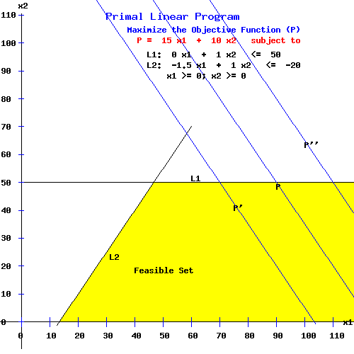
the next example has an unbounded primal solution, with an unfeasible dual problem.
Primal Linear Program
Maximize the Objective Function (P)
P = 15 x1 + 10 x2 subject to
L1: 0 x1 + 1.0 x2 <= 50
L2: -1.5 x1 + 1.0 x2 <= -20
x1 >= 0; x2 >= 0
|
Dual Linear Program
Minimize the Objective Function (D)
D = 50 y1 - 20 y2 subject to
G1: 0 y1 - 1.5 y2 >= 15
G2: 1.0 y1 + 1.0 y2 >= 10
y1 >= 0; y2 >= 0
|
To solve this problem using the primal simplex algorithm, set up the initial tableau as usual:
| Tableau0 |
| |
b0 |
x01 |
x02 |
s01 |
s02 |
e3 |
row
sum |
b / x1 |
| L01 |
50 | 0.00 |
1.00 | 1.00 |
0.00 | 0.00 |
52 | infinity |
| L02 |
-20 | -1.5 |
1.00 | 0.00 |
1.00 | 0.00 |
-19.5 | 13.3 |
| P0 |
0.00 | -15 |
-10 | 0.00 |
0.00 | 1.00 |
-24 | |
Phase 0: Complete since there are no artificial variables.
Phase I: Since b02 = -20 <= 0, the algorithm is in Phase I.
Goal: Generate a feasible program so that b >= 0.
A. In Tableau0:
1. Select a target row, r, with br < 0: b02 = -20, r = 2.
2. Select any column, col, with a negative entry in row 2 as the pivot column: col = 1 associated with variable x1, x2,1 = -1.5.
3. Compute the ratios bi / xi,3 as per the last column.
Select the row with the smallest positive ratio: L2 = 13.3. Thus x2,1 = -1.5 is the pivot; slack variable s2 will leave the basis; x2 will enter the basis.
To Create Tableau1:
4. Compute row L12 = L02 / (-1.5).
5. Subtract multiples of row L12 from all other rows of Tableau0 so that x12 = e2 in Tableau1.
| Tableau1 |
| |
b1 |
x11 |
x12 |
s11 |
s12 |
e3 |
row
sum |
b / x2 |
| L11 = L01 - 0 L12 |
50 | 0.00 |
1.00 | 1.00 |
0.00 | 0.00 |
52 | 50 |
| L12 = L02 / (-1.5) |
13.333 | 1.00 |
-0.667 | 0.00 |
-0.667 | 0.00 |
13 | -20 |
| P1 = P0 - (-15) L12 |
200 | 0.00 |
-20.005 | 0.00 |
-10.005 | 1.00 |
171 | |
Phase I is complete: b = ß >= 0.
Phase II. Try to increase the value of P = µ = 200 by eliminating negative entries from the last row.
A. In Tableau1:
1. Since the coefficient of x2 in the last row, -20.005, is the most negative, x2 will enter the basis.
2. Compute the ratios bi / xi,2 as per the last column: select the row with the smallest positive ratio, L1 = 50. Thus x1,2 = 1.0 is the pivot , and slack variable s1 will leave the basis.
B. To create Tableau2:
3. Compute row L21 by dividing row L11 by the pivot = 1.0.
4. Subtract multiples of row L21 from all other rows of Tableau1 so that x22 = e1 in Tableau2.
| Tableau2 |
| |
b2 |
x21 |
x22 |
s21 |
s22 |
e3 |
row
sum |
b / s2 |
| L21 = L11 / 1 |
50 | 0.00 |
1.00 | 1.00 |
0.00 | 0.00 |
52 | infinity |
| L22 = L12 - (-0.667) L21 |
46.667 | 1.00 |
0.00 | 0.667 |
-0.667 | 0.00 |
47.67 | -71.46 |
| P2 = P1 - (-20.005) L21 |
1200.25 | 0.00 |
0.00 | 20.005 |
-10.005 | 1.00 |
1211.25 | |
Phase I is complete: b = ß >= 0.
Phase II. The coefficient of s2 = -10.005 in the last row.
A. In Tableau2:
1. Since the coefficient of s2 in the last row is -10.005, s2 will enter the basis.
2. Compute the ratios bi / si,2 as per the last column. The smallest positive ratio, L1 = infinity. No suitable ratio exists. ==>> P is unbounded.
As the following diagram shows, the objective function P is unbounded since it intersects the feasible set for any large positive number = P.
Degeneracy and Cycling.
The primal simplex algorithm calculates a sequence of tableaus. The algorithm breaks down when in a given Tableauk:
a zero entry appears in the ß column and/or in the Ø row for a variable that is not one of the standard basis variables.
The example from N. Paul Loomba (152) illustrates the degeneracy problem.
Primal Linear Program
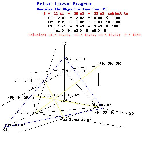
Maximize the Objective Function (P)
P = 22 x1 + 30 x2 + 25 x3 subject to
L1: 2 x1 + 2 x2 + 0 x3 <= 100
L2: 2 x1 + 1 x2 + 1 x3 <= 100
L3: 1 x1 + 2 x2 + 2 x3 <= 100
x1 >= 0; x2 >= 0; x3 >= 0
|
The three dimensional diagram shows how the three restraining planes intersect at the point (33.33, 16.67, 16.67).
P-Plane passing through (75, 0, 0), (0, 55, 0), (0, 0, 66), and (33.33, 16.67, 16.67) when P = 1650
L1-plane passing through (50, 0, 0), (0, 50, 0) perpendicular to the X1-X2 plane
L2-plane passing through (50, 0, 0), (0, 100, 0), and (0, 0, 100)
L3-plane passing through (100, 0, 0), (0, 50, 0), and (0, 0, 50)
L1 & L2 planes intersect along the line through (50, 0, 0), (33.33, 16.67, 16.67), and (0, 50, 50)
L1 & L3 planes intersect along the line through (50, 0, 25), (33.33, 16.67, 16.67), and (0, 50, 0)
L2 & L3 planes intersect along the line through (33.33, 33.33, 0), (33.33, 16.67, 16.67), and (33.33, 0, 33.33)
With P = 1650, the P-plane intersects the primal feasible set only at the point (33.33, 16.67, 16.67).
|
This problem's initial tableau is:
| Tableau0 |
| |
b0 |
x01 |
x02 |
x03 |
s01 |
s02 |
s03 |
e4 |
row
sum |
b / x2 |
| L01 |
100 | 2.0 |
2.0 | 0.0 |
1.00 | 0.00 |
0.00 | 0.00 |
105.0 | 50.0 |
| L02 |
100 | 2.0 |
1.0 | 1.0 |
0.00 | 1.00 |
0.00 | 0.00 |
105.0 | 100.0 |
| L03 |
100 | 1.0 |
2.0 | 2.0 |
0.00 | 0.00 |
1.00 | 0.00 |
106.0 | 50.0 |
| P0 |
0.00 | -22 |
-30 | -25 |
0.00 | 0.00 |
0.00 | 1.00 |
-76.00 | |
The pivot column is 2, since -30 is the most negative Ø entry; the pivot row is 1, since 50.0 is the smallest b / x2 ratio; and the pivot = 2. However, row L03 also has a 50.0 = b / x2 ratio. Applying the primal simplex algorithm yields the next tableau:
| Tableau1 |
| |
b1 |
x11 |
x12 |
x13 |
s11 |
s12 |
s13 |
e4 |
row
sum |
b / x3 |
| L11 = L01 / 2 |
50.00 | 1.00 |
1.00 | 0.00 |
0.50 | 0.00 |
0.00 | 0.00 |
52.50 | infinity |
| L12 = L02 - 1 L11 |
50.00 | 1.00 |
0.00 | 1.00 |
-0.50 | 1.00 |
0.00 | 0.00 |
52.50 | 50.0 |
| L13 = L03 - 2 L11 |
0.00 | -1.00 |
0.00 | 2.00 |
-1.00 | 0.00 |
1.00 | 0.00 |
1.00 | 0.00 |
| P1 = P0 - (-30) L11 |
1500.00 | 8.00 |
0.00 | -25.00 |
15.00 | 0.00 |
0.00 | 1.00 |
1499.00 | |
The variable x2 has replaced s1 in the basis. But ß3 = b13 = 0.0 -- the tableau is degenerate.
Charnes perturbation procedure resolves the degeneracy problem by adding small constants to the RHS of the constraints. Letting € = .1, the RHS vector b becomes:
bp = (b1+€, b2+€2, b3+€3)'
The perturbed problem's initial tableau is:
| Tableau0 |
| |
b0 |
x01 |
x02 |
x03 |
s01 |
s02 |
s03 |
e4 |
row
sum |
b / x2 |
| L01 |
100.1 | 2.0 |
2.0 | 0.0 |
1.00 | 0.00 |
0.00 | 0.00 |
105.1 | 50.05 |
| L02 |
100.01 | 2.0 |
1.0 | 1.0 |
0.00 | 1.00 |
0.00 | 0.00 |
105.01 | 100.01 |
| L03 |
100.001 | 1.0 |
2.0 | 2.0 |
0.00 | 0.00 |
1.00 | 0.00 |
106.001 | 50.0005 |
| P0 |
0.00 | -22 |
-30 | -25 |
0.00 | 0.00 |
0.00 | 1.00 |
-76.00 | |
The pivot column is 2, since -30 is the most negative Ø entry; the pivot row is 3, since 50.005 is the smallest b / x2 ratio; and the pivot = 2. Applying the primal simplex algorithm yields the next tableau:
| Tableau1 |
| |
b1 |
x11 |
x12 |
x13 |
s11 |
s12 |
s13 |
e4 |
row
sum |
b / x1 |
| L11 = L01 - 2 L13 |
0.099 | 1.00 |
0.00 | -2.00 |
1.00 | 0.00 |
-1.00 | 0.00 |
-0.901 | 0.099 |
| L12 = L02 - 2 L13 |
50.0095 | 1.50 |
0.00 | 0.00 |
0.00 | 1.00 |
-0.50 | 0.00 |
52.0095 | 33.3397 |
| L13 = L03 / 2 L11 |
50.0005 | 0.50 |
1.00 | 1.00 |
0.00 | 0.00 |
0.50 | 0.00 |
53.0005 | 100.001 |
| P1 = P0 - (-30) L11 |
1500.015 | -7.00 |
0.00 | 5.00 |
0.00 | 0.00 |
15.00 | 1.00 |
1514.015 | |
Because of the b0 vector was perturbed, no zero appears in the b1 vector.
The variable x2 has replaced the slack variable s3 in the basis.
The pivot column is 1, since -7 is the most negative Ø entry; the pivot row is 1, since 0.0990 is the least positive b / x1 ratio; and the pivot = 1. Applying the primal simplex algorithm yields:
| Tableau2 |
| |
b2 |
x21 |
x22 |
x23 |
s21 |
s22 |
s23 |
e4 |
row
sum |
b / x3 |
| L21 = L11 / 1 |
0.099 | 1.00 |
0.00 | -2.00 |
1.00 | 0.00 |
-1.00 | 0.00 |
-0.901 | -0.0495 |
| L22 = L12 - 1.5 L21 |
49.861 | 0.00 |
0.00 | 3.00 |
-1.50 | 1.00 |
1.00 | 0.00 |
53.361 | 16.6203 |
| L23 = L13 - 0.5 L21 |
49.951 | 0.00 |
1.00 | 2.00 |
-0.50 | 0.00 |
1.00 | 0.00 |
53.451 | 24.9755 |
| P1 = P0 - (-7) L21> |
1500.708 | 0.00 |
0.00 | -9.00 |
7.00 | 0.00 |
8.00 | 1.00 |
1507.080 | |
The variable x1 has replaced the slack variable s1 in the basis.
The pivot column is 3, since -9 is the most negative Ø entry; the pivot row is 2, since 16.6201 is the least positive b / x3 ratio; and the pivot = 3. Applying the primal simplex algorithm yields:
| Tableau3 |
| |
b3 |
x31 |
x32 |
x33 |
s31 |
s32 |
s33 |
e4 |
row
sum |
|
| L31 = L21 - (-2) L32 |
33.3397 | 1.00 |
0.00 | 0.00 |
0.00 | 0.6667 |
-0.3333 | 0.00 |
34.673 | |
| L32 = L22 / 2 |
16.6203 | 0.00 |
0.00 | 1.00 |
-0.50 | 0.3333 |
0.3333 | 0.00 |
17.787 | |
| L33 = L23 - 2 L32 |
16.7103 | 0.00 |
1.00 | 0.00 |
0.50 | -0.6667 |
0.3333 | 0.00 |
17.877 | |
| P1 = P0 - (-9) L32> |
1650.291 | 0.00 |
0.00 | 0.00 |
2.50 | 3.00 |
11.00 | 1.00 |
1667.791 | |
The variable x3 replaces the slack variable s3 in the basis. The basis consists of all three primal variables, x1, x2, and x3.
The last tableau contains the solutions to the primal and dual perturbed problems. Letting:
| B | = |
| s31 |
s31 |
s33 |
e4 |
| 0.00 |
0.6667 |
-0.3333 |
0.00 |
| -0.50 |
0.3333 |
0.3333 |
0.00 |
| 0.50 |
-0.6667 |
0.3333 |
0.00 |
| 2.50 |
3.00 |
11.00 |
1.00 |
|
The solution to the original primal problem is:
(x1, x2, x3, P)' = B * (b1, b2, b3, 0)' = B *(100, 100, 100, 0) = (33.33, 16.67, 16.67, 1650.0)'.
The solution to the dual problem is:
(y1, y2, y3, D)' = (2.5, 3.00, 11.0, 1650.0)'.
Linear Programming References.
- Budnick, Frank S., Richard Mojena, and Thomas E. Vollmann. Principles of Operations Research for Management. Homewood: Irwin, 1977.
- Dantzig, G., A. Orden, and P. Wolfe. "The Generalized Simplex Method for Minimizing a Linear Form under Inequality Restraints." Pacific Journal of Mathematics. 8, (1955): 183-195.
-
Dantzig, George B. Linear Programming and Extensions. Princeton: Princeton U P, 1963.
-
Dorfman, R., P. Samuelson, and R. Solow. Linear Programming and Economics Analysis. New York: McGraw-Hill, 1958.
-
Hadley, G. Linear Algebra. Reading, Mass.: Addison-Wesley, 1961.
-
Hadley, G. Linear Programming. Reading, Mass.: Addison-Wesley, 1962.
- Hillier, Frederick S. and Gerald J. Lieberman. Operations Research.. 2nd ed. San Francisco: Holden-Day, 1974.
-
Karlin, S. Mathematical Methods in the Theory of Games and Programming. Vols. I & II. Reading, Mass.: Addison-Wesley, 1959.
- Loomba, N. Paul. Linear Programming: An Introductory Analysis. New York: McGraw-Hill, 1964.
- Press, William H., Brian P. Flannery, Saul A. Teukolsky, and William T. Vetterling. Numerical Recipes: The Art of Scientific Computing. Cambridge: Cambridge UP, 1989.
-
Saaty, Thomas L. Mathematical Methods of Operations Research. New York: McGraw-Hill, 1959.
- Sierksma, Gerard. Linear and Integer Programming: Theory and Practice. 2nd ed. New York: Marcel Dekker, 2002.
-
Sposito, Vincent. Linear and Nonlinear Programming. Ames, Iowa: Iowa UP, 1975.
-
Sposito, Vincent. Linear Programming with Statistical Applications. Ames, Iowa: Iowa UP, 1989.
-
Strang, Gilbert. Linear Algebra and Its Applications.3rd ed. San Diego: Harcourt, 1988.
-
Restrepo, Rodrigo A. Theory of Games and Programming: Mathematics Lecture Notes. Vancouver: University of B.C., 1967.
-
Restrepo, Rodrigo A. Linear Programming and Complementarity. Vancouver: University of B.C., 1994.
-
Taha, Hamdy A. Operations Research: An Introduction. 2nd ed. New York: MacMillan, 1976.
- Wagner, Harvey M. Principles of Management Science: With Applications to Executive Decisions. 2nd ed. Englewood Cliffs: Prentice-Hall, 1975.
- Wagner, Harvey M. Principles of Operations Research: With Applications to Managerial Decisions. 2nd ed. Englewood Cliffs: Prentice-Hall, 1975.
- Wu, Nesa, and Richard Coppins. Linear Programming and Extensions. New York: McGraw-Hill, 1981.
|
|