
|
|
|
|
|
|
|
|
|
|
         
|
|
Egwald Mathematics: Linear Algebra
Egwald's popular web pages are provided without cost to users.
linear differential equations | matrix representation | eigenvector basis | example problems | general solution - eigenvector basis A System of Linear Differential Equations. A system of linear differential equations can be expressed as:
where xi(t) is a function of time, i = 1, . . . n, and the matrix of constant coefficient is A = [ai,j]. This system of linear differential equations is called autonomous because the coefficients of A are not explicit functions of time. Example.
Objective: obtain formulae for the functions xi(t), i = 1, . . . n. To obtain explicit formulae for the functions xi(t), i = 1, . . . n, one must find the complete set of eigenvalues and eigenvectors of the matrix A. If A has repeated eigenvalues, one might also need to compute their generalized eigenvectors. The eigenvalues and eigenvectors of A can be real numbers and vectors in Rn, or complex numbers and vectors in Cn. Matrix Representation. The same problem expressed in matrix and vector form is:
where x(t)T = (x1(t), x2(t), . . . . xn(t)) is the vector of unknown functions of time, and A = [ai, j] is the matrix of coefficients.
The Eigenvectors of A Form a Basis of Rn. If the eigenvectors of the matrix A of dimension n form a basis of Rn, then A can be diagonalized as: A = S * D * S(-1) where D is a diagonal matrix formed from the eigenvalues of A, and S is matrix whose columns are their associated eigenvectors listed in the same order as the eigenvalues in D. Example Problem #1: A with two negative eigenvalues. Find equations xT(t) = (x1(t), x2(t)) for the system dx/dt = A * x, with x(0) = x0 = (x01, x02), where
In matrix form, this system of linear differential equations is:
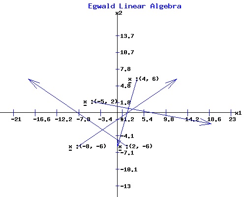
where I dropped the reference to time t. The values of dxT/dt = (dx1/dt, dx2/dt) depend on the matrix A, and on the values of xT = (x1, x2). For example:
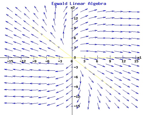
In the following diagram, the values of dx/dt and x are plotted for four sets of values in the x1-x2 plane. The vector dx/dt begins at x with its direction and magnitude provided by the coefficients of the vector dx/dt.
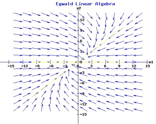
If one starts at t = 0 at the initial point x0T = (x01, x02), one can follow the trajectory of x(t) as time t proceeds as given by dxT(t)/dt = (dx1(t)/dt, dx2(t)/dt). The next diagram shows the normalized vectors of dx(t)/dt at points of xT = (x1, x2). These vectors represented as arrows provide a picture of a vector field in the x1-x2 plane generated by the system of linear differential equations. To obtain a rough trajectory of the solution vector x(t), start at an initial point x0, (t = 0), and follow the arrows as t increases in value.
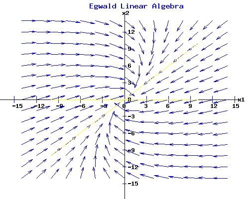
The pattern that the arrows make in the diagram depends on the values of the coefficients of the matrix A. From any initial point x0, the trajectory of xT(t) = (x1(t), x2(t)) converges over time to the origin oT = (0, 0) for this particular matrix A. The origin is an equilibrium point for any matrix since A * o = o. For this linear differential equation system, the origin is a stable node because any trajectory proceeds to the origin over time. Solution to dx(t)/dt = A * x(t). The solution to a system of linear differential equations involves the eigenvalues and eigenvectors of the matrix A.
This matrix has two distinct eigenvalues, µ1 = -4 and µ2 = -2, with corresponding linearly independent eigenvectors, v1T = (1, 0) and v2T = (1, 1). The general solution for given constants c1 and c2 is:
x(t) = c1 * e�1*t * v1 + c2 * e�2*t * v2, or where ef(t) is the exponential of the function f(t). One uses the constant vector cT = (c1, c2) to determine the initial point x0T = (x01, x02) of a particular solution trajectory, xT(t) = (x1(t), x2(t)). Expanding:
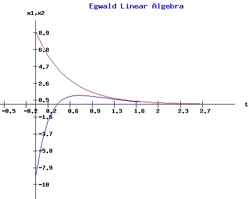
Considering each variable with the initial conditions xT(0) = x0T = (-9, 9):
Solving for the constants yields c1 = -18, c2 = 9.
Starting at the initial point x0T = (-9, 9), the evolution of x1(t) in blue and x2(t) in red appear below. Both curves converge to 0. Their formulae involve the exponential of the two negative eigenvalues of A, µ1 = -4 and µ2 = -2, multiplied by the time variable t. As t increases in value, x1(t) and x2(t) are both forced to 0, because for any positive constant k, e-k*t converges to 0 as the variable t increases in value. Moreover, e-k*t converges to 0 more quickly if the magnitude of k is increased.
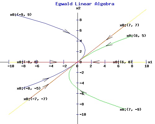
The phase portrait of the solution vector xT(t) = (x1(t), x2(t)) appears in the next diagram. The trajectories from eight initial points are curves in the x1-x2 plane that terminate at the origin.
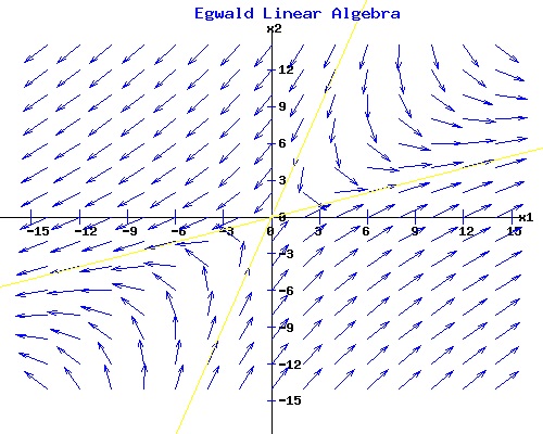
Trajectories that begin on the yellow lines through the eigenvectors, v1T = (1, 0) and v2T = (1, 1) move directly toward the origin. Example Problem #2. A with one negative and one positive eigenvalue. Find equations xT(t) = (x1(t), x2(t)) for the system dx/dt = A * x, with x(0) = x0 = (x01, x02), where
This matrix has two distinct eigenvalues, µ1 = 4 and µ2 = -4, with corresponding linearly independent eigenvectors, v1T = (3, 1) and v2T = (1, 3). The general solution for given constants c1 and c2 is: x(t) = c1 * e4*t * v1 + c2 * e-4*t * v2. Considering each variable with the initial conditions xT(0) = x0T = (x01, x02):
The phase diagram for this system is:
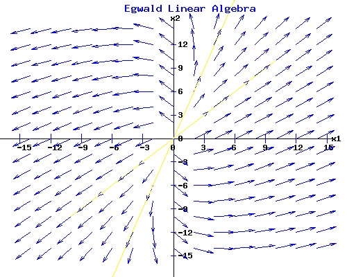
A trajectory that starts along the yellow line passing through the eigenvector v1T = (3, 1) associated with the positive eigenvalue µ1 = 4 moves directly away from the origin. A trajectory that starts along the yellow line passing through the eigenvector v2T = (1, 3) associated with the negative eigenvalue µ2 = -4 moves directly to the origin. All other trajectories diverge from the origin. The line passing through the eigenvector v2T = (1, 3) is called the separatrix. The origin in this situation as determined by the matrix A is called a saddle point. Example Problem #3. A with two positive eigenvalues. Find equations xT(t) = (x1(t), x2(t)) for the system dx/dt = A * x, with x(0) = x0 = (x01, x02), where
This matrix has two distinct eigenvalues, µ1 = 4 and µ2 = 2, with corresponding linearly independent eigenvectors, v1T = (1, 1) and v2T = (1, 3). The general solution for given constants c1 and c2 is: x(t) = c1 * e4*t * v1 + c2 * e2*t * v2. Considering each variable with the initial conditions xT(0) = x0T = (x01, x02):
The phase diagram for this system is:
A trajectory that starts along the yellow line passing through either eigenvector v1T = (1, 1) or v2T = (1, 3) moves directly away from the origin. All other trajectories diverge from the origin. The origin in this situation as determined by the matrix A is called an unstable node. General Solution: The Eigenvectors of A Form a Basis of Rn. If the eigenvectors of the matrix A of dimension n form a basis of Rn, then A can be diagonalized as: A = S * D * S(-1) where D is a diagonal matrix formed from the eigenvalues of A, and S is a matrix whose columns are their associated eigenvectors listed in the same order as the eigenvalues in D. The system of linear differential equations can be expressed as:
Define the new vector of variables y(t) as:
Since:
and
the decoupled system of differential equations is:
If {µ1, µ2, . . . µn) are the eigenvalues of A, then:
and the individual equations of the decoupled system of dimension n are:
Any one-dimensional equation of the form has the solution So the decoupled system has the solution:
In matrix form this is:
To get the general solution for the system dx/dt = A *x, x(0) = x0, define the vector of constants cT = (c1, c2, . . . cn) as: c = S(-1) * x0 = y0. Also, let {v1, v2, . . . vn} be the set of linearly independent eigenvectors associated with the eigenvalues {µ1, µ2, . . . µn), so that: S = [v1 | v2 | . . . | vn]. Multiplying the following equation by S:
yields:
The general solution of the system of linear differential equations is:
The Matrix Exponential of a Diagonalizable Matrix The square matrix A of dimension n is diagonalizable if: A = S * D * S(-1) where D is the diagonal matrix of eigenvalues {µ1, µ2, . . . µn), and S = [v1 | v2 | . . . | vn], ie the columns of S are the linearly independent eigenvectors. Powers of A: Ak. The kth power of A can be written as: Ak = (S * D * S(-1)) * (S * D * S(-1)) * . . . (S * D * S(-1)) = S * Dk * S(-1). Power Series of et. The power series expansion of et is: et = 1 + t + tt/2! + t3/3! + . . . Power Series of eA*t. The power series expansion of eA*t is: eA*t = 1 + A*t + (A*t)2/2! + (A*t)3/3! + . . . eA*t = I + (S * (D*t) * S(-1)) + (S * (D*t)2 * S(-1))/2! + (S * (D*t)3 * S(-1))/3! + . . . eA*t = S * (I + (D*t) + (D*t)2/2! + (D*t)3/3! + . . . ) * S(-1) = S * eD*t * S(-1) The general solution of the system of linear differential equations in terms of the matrix exponential of A is:
where the matrix exponential of the diagonal matrix D*t is:
The Eigenvectors and Generalized Eigenvectors of A Form a Basis of Rn. The Matrix Exponential of a Jordan Matrix. Suppose A is a square matrix of dimension 2, with a repeated eigenvalue µ, an eigenvector v1, and a generalized eigenvector v2. Form the matrix S = [v1 | v2], ie its columns are the linearly independent vectors v1 and v2. Let J be the Jordan matrix:
The Jordan Normal decomposition of A is: A = S * J * S(-1). The power series expansion of eA*t is: eA*t = S * (I + (J*t) + (J*t)2/2! + (J*t)3/3! + . . . ) * S(-1) = S * eJ*t * S(-1) where the matrix exponential of the Jordan matrix J*t is:
General Solution: The Eigenvectors and Generalized Eigenvectors of A Form a Basis of Rn. The general solution of the system of linear differential equations in terms of the matrix exponential of A is:
Defining the vector of constants cT = (c1, c2, . . . cn) as: c = S(-1) * x0. the general solution is:
since eJ * 0 = I, the identity matrix. Example Problem #4. A with a repeated negative eigenvalue. Find equations xT(t) = (x1(t), x2(t)) for the system dx/dt = A * x, with x(0) = x0 = (x01, x02), where
This matrix has the characteristic equation: f(µ) = µ2 - trace(A) * µ + det(A) = µ2 + 4 * µ + 4, with a repeated eigenvalue root, µ1 = -2 and µ2 = -2. Compute the eigenvector(s) v1, 2 by solving the system of equations (A - (-2) * I) * v = 0:
Using the echelon algorithm, or just noticing that equations e1 and e2 are the same, one determines that matrix A has only one eigenvector, v1T = (1, 1). To find the general solution for this problem, one must also compute a generalized eigenvector v2T associated with v1T. Solve:
(A - (-2) * I)*v2 = v1, or
Using the echelon algorithm form, one obtains:
The particular solution vTp = (-1, 0) = v2 is the generalized eigenvalue of the matrix A associated with the pair of equal eigenvalues µ1,2 = -2, while the homogeneous solution vh is the eigenvector v1. Therefore:
The general solution for given constants cT = (c1, c2) is: x(t) = S * eJ*t * c Considering each variable with the initial conditions xT(0) = x0T = (x01, x02):
The phase diagram for this system is:
A trajectory that starts along the yellow line passing through the eigenvector v1T = (1, 1) moves directly towards the origin. All other trajectories converge to the origin over time, including trajectories that start along the yellow line through the generalized eigenvector v2T = (-1, 0). The origin in this situation as determined by the matrix A is called a stable degenerate node. Example Problem #5. A with a repeated positive eigenvalue. Find equations xT(t) = (x1(t), x2(t)) for the system dx/dt = A * x, with x(0) = x0 = (x01, x02), where
This matrix has a repeated eigenvalue, µ1 = 2 and µ2 = 2, with only one eigenvector, v1T = (1, -1). To find the general solution for this problem one must compute a generalized eigenvector associated with v1T. On the matrix web page, I determined that the generalized eigenvector v2T = (1, 0) for this particular matrix A. Therefore:
The general solution for given constants cT = (c1, c2) is: x(t) = S * eJ*t * c Considering each variable with the initial conditions xT(0) = x0T = (x01, x02):
The phase diagram for this system is:
A trajectory that starts along the yellow line passing through the eigenvector v1T = (1, -1) moves directly away from the origin. All other trajectories diverge from the origin, including trajectories that start along the yellow line through the generalized eigenvector v2T = (1, 0). The origin in this situation as determined by the matrix A is called an unstable degenerate node. Phase Diagram of a General Two by Two Matrix The matrices in the examples above had real eigenvalues and real eigenvectors. However, matrices can also have complex valued eigenvalues and complex valued eigenvectors. The patterns of the phase diagrams with complex eigenvalues differ from the ones with real eigenvalues.
This matrix has the characteristic equation: f(µ) = µ2 - 0 * µ + 1 with eigenvalues: µ1 = 0 + 1 * i, µ2 = 0 + -1 * i The phase diagram for this system is:
Use the form below to plot the phase diagram of some other 2 by 2 matrix. Classification of the Equilibrium Point at the Origin The origin is an equilibrium point for any system of linear differential equations with coefficient matrix A because A * o = o. One can examine the behaviour of the solution vector x(t) near the origin o by analyzing the eigenvalues and eigenvectors of A. The general 2 by 2 matrix:
has trace(A) = a + d, and det(A) = a*d - b*c. Its characteristic equations is: f(µ) = µ2 - trace(A) * µ + det(A) Factoring this quadratic equation yields the pair of eigenvalues, µ1 and µ2, where:
µ1 = {trace(A) + sqrt[trace(A) * trace(A) - 4 * det(A)]} / 2 , and
det(A) = µ1 * µ2, and If the discriminant: disc(A) = trace(A) * trace(A) - 4 * det(A) is positive, µ1 and µ2 are real and distinct. Also, if det(A) > 0, µ1 and µ2 have the same sign. Furthermore, if trace(A) is negative, µ1 and µ2 are negative, and the origin is a stable node.. But, if trace(A) is positive, µ1 and µ2 are positive, and the origin is an unstable node.
If the determinant of A, det(A), is negative, then disc(A) > 0 and µ1 and µ2 are real and have opposite signs. The origin is a saddle point.
If the discriminant: disc(A) = trace(A) * trace(A) - 4 * det(A) is negative, the eigenvalues of A, µ1 and µ2, are complex conjugates:
µ1 = ρ + i * ω If real(µ1,2) = ρ < 0, then the origin is a stable focus with trajectories spiralling inwards toward o;
If real(µ1,2) = ρ > 0, then the origin is an unstable focus with trajectories spiralling outward from o.
If real(µ1,2) = ρ = 0, the origin is an neutrally stable center with trajectories ellipses about the origin o.
If the discriminant: disc(A) = trace(A) * trace(A) - 4 * det(A) is zero, the eigenvalues of A, µ1 and µ2, are real and equal. If the matrix A has only one distinct eigenvector direction, the origin is a degenerate node. In the examples below, with µ1,2 = -2, the origin is a degenerate stable node with trajectories that arc toward the origin o. With µ1,2 = 2, the origin is a degenerate unstable node with trajectories that arc away from the origin o.
If the discriminant: disc(A) = trace(A) * trace(A) - 4 * det(A) is zero, the eigenvalues of A, µ1 and µ2, are real and equal. If the matrix A has two distinct eigenvector directions, the origin is a star node. In the examples below, with µ1,2 = -2, the origin is a stable star node with trajectories that move directly toward the origin o. With µ1,2 = 2, the origin is a unstable star node with trajectories that move directly away from the origin o.
If the determinant of A, det(A), is zero, at least one the eigenvalues is zero. If µ1 = 0 and µ2 is not 0, there is a line of equilibrium points passing through the eigenvector corresponding to the zero eigenvector. All other trajectories are parallel to the line through the other eigenvector. If µ2 < 0, the line of equilibrium points is stable. If µ2 > 0, the line of equilibrium points is unstable.
If the determinant of A is zero and µ1 = 0 and µ2 = 0, two possibilities exist. If A is the zero matrix, every point is an equilibrium point. Otherwise, there is a line of equilibrium points passing through the eigenvector corresponding to one zero eigenvalue. All other trajectories are parallel to this line, running in opposite directions on either side of the line of equilibrium points.
Click to pop a new window with a summary of this analysis: Classification of the Equilibrium Point at the Origin. References.
|
||||||||||||||||||||||||||||||||||||||||||||||||||||||||||||||||||||||||||||||||||||||||||||||||||||||||||||||||||||||||||||||||||||||||||||||||||||||||||||||||||||||||||||||||||||||||||||||||||||||||||||||||||||||||||||||||||||||||||||||||||||||||||||||||||||||||||||||||||||||||||||||||||||||||||||||||||||||||||||||||||||||||||||||||||||||||||||||||||||||||||||||||||||||||||||||||||||||||||||||||||||||||||||||||||||||||||||||||||||||||||||||||||||||||||||||||||||||||||||||||||||||||||||||||||||||||||||||||||||||||||||||
|

