| |
Egwald Economics: Microeconomics
Derivation of the Model: Oligopoly / Public Firm
by
Elmer G. Wiens
Egwald's popular web pages are provided without cost to users.
Follow Elmer Wiens on Twitter:

Bonus System: Profit, Industry Output, and Own Revenue
|
Notation:
|
|---|
|
Q = sum(q) = sum(q0,q1,...qn); qi = firm i's output; i = 0 for public
firm
|
|
D(Q) = the industry's inverse demand schedule: downward slopping
|
|
Ci(qi) = the cost schedule for the ith firm: textbook U-shaped average cost curves
|
|
Income of Public Firm Managers:
|
|---|
I0(Q) = b1*[D(Q)*q0 - C0(q0)] + b2*Q + b3*[D(Q)*q0] b1, b2, b3 >= 0 bonus weights
I0(Q) = b1*prof0(q0) + b2*Q + b3*[D(Q)*q0]
|
|
Income(Profit) of Private firms:
|
|---|
|
Ii(Q) = D(Q)*qi - Ci(qi) = profi(qi)
| |
Income Maximization: First Order Conditions:
|
|---|
|
Public Firm:
|
|---|
dI0/dq0 = b1*[D'(Q)*q0 + D(Q) - C0'(q0)] + b2 + b3*[D'(Q)*q0 + D(Q)] = 0
dI0/dq0 = b1*[mrf0(q0) - mc0(q0)] + b2 +b3*mrf0(q0) = 0
mrf0(q0) = D'(Q)*q0 + D(Q) GAP = mc0(q0) - mrf0(q0)
|
|
Private Firms: Cournot Behaviour
|
|---|
|
dIi/dqi = mrfi(qi) - mci(qi) = 0 mrfi(qi) = D'(Q)*qi + D(Q)
|
|
Income Maximization: Second Order Conditions:
|
|---|
|
Public Firm:
|
|---|
|
ddI0/ddq0 = b1 * [mrf0'(q0) - mc0'(q0)] + b3 * mrf0'(q0)] < 0
|
|
Private Firms: Cournot Behaviour
|
|---|
|
ddIi/ddqi = mrfi'(qi) - mci'(qi) < 0
| |
The Jacobian used in the Gradient and Newton's Methods for solving the system of first order equations uses the second order formulae plus the cross derivatives:
|
|---|
|
Public Firm:
|
|---|
|
ddI0/dq0dqi = b1 * mrf0'(q0) + b3 * mrf0'(q0)]
|
|
Private Firms:
|
|---|
|
ddIi/dqjdqi = mrfi'(qi) i != j
|
|
Linear Programming Problem
|
|---|
|
maximize z = b1 - b2 - b3
| b1, b2, b3 >= 0 |
| | b3*mrf0(q0) | >= 0 |
| b1*(-GAP) | + b2 | + b3*mrf0(q0) |
= 0 |
| b1*prof0(q0) | + b2*Q | + b3*[D(Q)*q0] |
= Total Bonus |
|
| Alternate Solution: System of Linear Equations
|
|---|
| mrf0(q0) > 0 | mrf0(q0) <= 0 |
|---|
b1*(-GAP) + b3*mrf0(q0) = 0
b1*prof0(q0)] + b3*[D(Q)*q0] = Total Bonus |
b1*(-GAP) + b2 = 0
b1*prof0(q0) + b2*Q = Total Bonus
|
|
| How does it work? |
|---|
| The 'government' adjusts 'THE GAP' - the difference between the g.f.'s marginal cost and marginal revenue - until it achieves the level of industry output that it wants. For each setting of 'THE GAP' it solves the linear programming problem for the bonus rates b1,b2,b3. Then it tells the managers that their bonus will be paid using those rates applied to the government firm's profit, industry's total output, and government firm's revenue, respectively. Notice that the 'government' does not need to know the government firm's cost structure, if it can iterate its choice of 'THE GAP.'
|
|
I. Maximize government firm's consumer + producer surplus
|
|---|
|
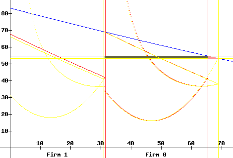
Suppose the 'government' wants the government firm to produce where marginal cost equals price. In the jargon of welfare economics, it wants to maximize consumer plus producer surplus flowing from the g.f.
In the diagram below, the red lines represent the equilibrium (1 private firm + 1 g.f.) at time t-1 with the GAPt-1 = 1.
qt-10 = 34.28, qt-11 = 31.60, price pt-1 = 54.95, total output Qt-1= 65.88
proft-10 = 611.75, revt-10 = 1883.63; proft-11 = 569.85, revt-11 = 1736.69
bt-11 = 0.0304, bt-12 = 0, bt-13 = 0.00076
The yellow lines represent the equilibrium at time t with the GAPt = 15.2.
qt0 = 38.03, qt1 = 31.19, price pt = 53.61, total output Qt = 69.22
proft0 = 567.90, revt0 = 2038.85; proft1 = 522.54, revt1 = 1672.33
bt1 = 0.0143, bt2 = 0, bt3 = 0.00568
Notice how the weight on g.f. profits, b1, decreases and the weight on g.f. revenue, b3, increases - with the increase in the GAP and the increase in total output.
Essentially, the government can adjust (search) the value of the GAP (or equivalently - the values of the weights b1, b2, b3) until it is satisfied with the resulting equilibrium.
|
|
There are many ways in which the government can arrive at the value of the GAP that it deems "best for its purposes." One way (brute force) would be to estimate econometrically all the equations underlying the lines and curves in the diagram above and then to compute the 'optimal' value of the GAP. Alternatively, the government could use the following iterative process that 'economizes' on the necessary information.
Iterative Process
Define the following variables:
DW1 = .5 * (qt0 - qt-10) * |pt - pt-1|
DW2 = (proft0 - proft-10) - (pt - pt-1) * qt-10 if (Qt - Qt-1) >= 0
DW2 = (proft0 - proft-10) - (pt - pt-1) * qt0 if (Qt - Qt-1) < 0
Then
DW = DW1 + DW2
is a measure of the change in welfare obtained directly from the government firm from the change in the GAP from GAPt-1 to GAPt.
DW1 estimates the change in consumer surplus that is not offset by a change in g.f producer surplus. DW1 = (approx.) the area of the small pink triangle in the diagram above.
DW2 estimates the change in g.f. producer surplus not offset by a change in consumer surplus. In the diagram above, the area of the olive rectangle estimates the producer surplus displaced by consumer surplus when price falls from pt-1 to pt.
Notice that no new information is required beyond that used in calculating the values of b1, b2, and b3 for a given value of the GAP.
Essentially, the government must solve the nonlinear process
DW(GAP) = 0
That is - find that value of the GAP where either an increase or decrease in the value of the GAP decreases the value of Consumer + Producer Surplus obtained directly from the government firm. Numerical Analysis provides many ways to solve such a nonlinear process.
|
|
II. Maximize industry's consumer surplus + g.f. producer surplus
|
|---|
|
The government can obtain a lower price - when private firms exhibit Cournot behavior or form a cartel - with the following modification to the above iterative method.
Define:
DW3 = (pt - pt-1) * (Qt-1 - qt-10) if (Qt - Qt-1) >= 0
DW3 = (pt - pt-1) * (Qt - qt0) if (Qt - Qt-1) < 0
DW = DW1 + DW2 - DW3
This process does not require any information on the profits and/or costs of the private firms. It tends to achieve an output level between the competitive level for the industry and the level using DW = DW1 + DW2.
|
|
Computing the Industry Equilibrium
|
|---|
|
When solving for the industry equilibrium (for a given set of behavioral assumptions and value of the GAP) for the firms, the model starts with the Gradient Method. Then it tries to switch to Newton's Method. If Newton's Method diverges (when private firms form a cartel), the model realizes it must drop a firm to obtain each firm's equilibrium.
|
|
The g.f. managers might obtain more or less than the desired total bonus if the industry is not in equilibrium, if the government does not adequately understand the demand conditions of the industry, and/or if the g.f. managers are not behaving 'optimally.' If, on average, this situation persists, the government needs to make some adjustments - which could include getting more competent g.f. managers.
|
|
Is the public firm minimizing cost?
|
|---|
| Notation |
|---|
l = (l0,l1,...,ln) L = sum(l);
k = (k0,k1,...,kn) K = sum(k);
wl(L) = labour supply schedule; wk(K) = capital supply schedule
fi(li,ki) = production function of the ith firm
ddfi(li,ki)/dlidli < 0 ddfi(li,ki)/dkidki < 0
ddfi(,)/dlidli * ddfi(,)/dkidki - ddfi(,)/dlidki * ddfi(,)/dkidli > 0
µi = Lagrangian multiplier for the ith firm, µi >= 0
|
| Income of Public Firm Managers: |
|---|
|
I0(l0,k0,µ0) = b1*[D(Q)*q0 - wl(L)*l0 - wk(K)*k0] + b2*Q + b3*D(Q)*q0 + µ0*[f0(l0,k0) - q0]
|
|
Income of Private Firms
|
|---|
|
Ii(li,ki,µi) = D(Q)*qi - wl(L)*li - wk(K)*ki + µi*[fi(li,ki) - qi]
|
|
Income Maximization: First Order Conditions:
|
|---|
|
Public Firm:
|
|---|
dI0/dl0 = b1*[-wl'(L)*l0 - wl(L)] + µ0*df0(l0,k0)/dl0 = 0
dI0/dk0 = b1*[-wk'(K)*k0 - wk(K)] + µ0*df0(l0,k0)/dk0 = 0
|
| Solve for µ0 / b1 |
|---|
|
[wl'(L)*l0 + wl(L)] / [df0(l0,k0)/dl0] = [wk'(K)*k0 + wk(K)] / [df0(l0,k0)/dk0]
|
|
Private Firms:
|
|---|
dIi/dli = -wl'(L)*li - wl(L) + µi*dfi(li,ki)/dli = 0
dIi/dki = -wk'(K)*ki - wk(K) + µi*dfi(li,ki)/dki = 0
|
| Solve for µi |
|---|
|
[wl'(L)*li + wl(L)] / [dfi(li,ki)/dli] = [wk'(K)*ki + wk(K)] / [dfi(li,ki)/dki]
|
Answer: Sure looks like it to me here. The input proportions, depending on the firm's production function, are the same for the public and private firms.
I'll let you work out the second order conditions yourself.
|
|---|
Back to Oligopoly / Public Firm Model
|
|