Egwald: Topics in Astronomy and Cosmology- The Curvature of Space

by

Elmer G. Wiens

Egwald's popular web pages are provided without cost to users.
Please show your support by joining Egwald Web Services as a Facebook Fan:
Follow Elmer Wiens on Twitter:

The Curvature of Space (Elemental Quantum Geometry)

Introduction

The cosmological principle states that the Universe is homogeneous and isotropic on large scales. Three cosmological models of the spatial constituent of the Universe that conform to this principle are hypersurfaces in a 4-dimensional space with uniform positive, zero, and negative curvature. The space of each model is specified by systems of coordinates that locate an object, and by a metric that determines the distance between objects

3D Euclidean Space: Zero Curvature (Κ = 0)

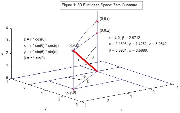
Figure 1:
An object can be located by its Cartesian coordinates, (x, y, z), or its spherical coordinates, (r, θ, φ), 0 <= r < ∞, 0 <= θ <= π, 0 <= φ <= 2 π.

An objects position vector is: l = (x, y, z) = (r*sin(θ)*cos(φ), r*sin(θ)*sin(φ), r*cos(θ)).

Its vector of differentials is dl = (dx, dy, dz), and the space’s metric is the dot product: dl*dl = dl² = (dx² + dy² + dz²) = dr² + r² [dθ² + sin²(θ) dφ²].

Setting ψ = r / R, this metric can be written as: dl² = R² (dψ² + ψ² [dθ² + sin²(θ) dφ²]).

All angles are measured in radians in the following examples.

4D Euclidean Space: Hypersurface with Positive Curvature (Κ = +1)

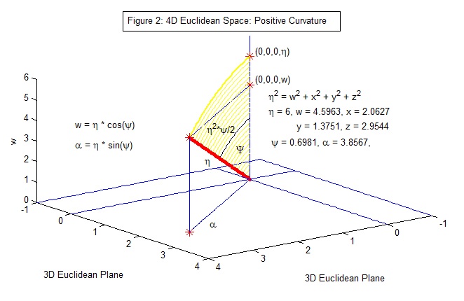
Figure 2: An object’s position vector is: l = (x, y, z, w) = (α*sin(θ)*cos(φ), α*sin(θ)*sin(φ), α*cos(θ), η*cos(ψ)), where α = η*sin(ψ) is the projection onto the 3D Euclidean space. These coordinates satisfy: η² = (x² + y² + z² + w²), and 0 <= ψ <= π, 0 <= θ <= π, 0 <= φ <= 2 π.

The W-axis is perpendicular to the 3D Euclidean surface. The radial vector η with length η at the polar angle ψ is projected onto the 3D surface as the vector α with length α. The coordinates of η satisfy η² * cos²(ψ) + η² * sin²(ψ) = η².

The area of the yellow sector is η² * ψ / 2.

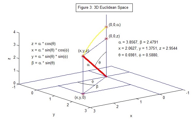
Figure 3: The radial vector α = (x, y, z) with length α is projected onto the 2D Euclidean plane at the polar angle θ as the vector β = (x, y, 0).

The 4D space's metric is: dl² = dη² + η² dψ² + η² sin²(ψ) [dθ² + sin²(θ) dφ²]. On a hypersphere of radius R with dη = 0, η² = R² = x² + y² + z² + w².

The metric: dl² = R² (dψ² + sin²(ψ) [dθ² + sin²(θ) dφ²]), where 0 <= r <= R * π.

Figure 4: The projection of the hypersphere onto the Z-W plane, where θ = 0, x = y = 0. Since ψ is the angle between the W-axis and the radius vector, the distance along the ψ coordinate geodesic is r = R * ψ. The (z, w) coordinates satisfy: z² + w² = R² * sin²(ψ) + R² * cos²(ψ) = R². The projection of the point on the sphere onto the Z-axis is α = R * sin(ψ). With R = 8, and ψ = 0.6981 these values are: z = α = R * sin(ψ) = 5.1421;   w = R * cos(ψ) = 6.1285 r = R * ψ = 5.5848 = the distance along the ψ geodesic = the line integral of the curve traced by the radius vectors from 0 to ψ. Yellow Area: R2 * ψ / 2 = 22.34

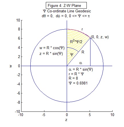In this context ψ can be called "the Euclidean angle" of the projection.

4D Pseudo-Euclidean Space: Hypersurface with Negative Curvature (Κ = -1)

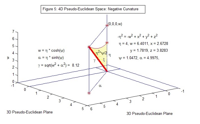
Figure 5: An object’s position vector is: l = (x, y, z, w) = (α*sin(θ)*cos(φ), α*sin(θ)*sin(φ), α*cos(θ), η*cosh(ψ)), where α = η*sinh(ψ) is the projection onto the 3D Euclidean space. These coordinates satisfy: -η² = (x² + y² + z² - w²), and 0 <= ψ < ∞, 0 <= θ <= π, 0 <= φ <= 2 π.

The coordinates of the vector γ = (α, w) satisfy: η² * sinh²(ψ) - η² * cosh²(ψ) = -η².

The area of the yellow sector is η² * ψ / 2.

Note: ψ is not the angle ζ = arccos(w/γ) = 0.663 subtended by the W-axis and the vector γ.

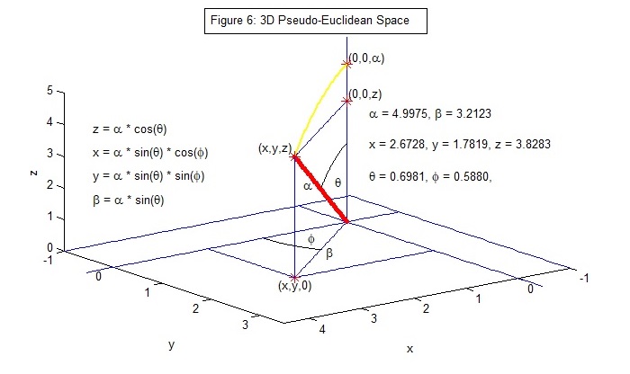
Figure 6: The radial vector α = (x, y, z) with length α is projected onto the 2D Pseudo-Euclidean plane at the polar angle θ as the vector β = (x, y, 0).

The 4D space's metric is: dl² = dη² + η² dψ² + η² sinh²(ψ) [dθ² + sin²(θ) dφ²]. On a hypersurface of radius R with dη = 0, -η² = -R² = x² + y² + z² - w².

The metric on the 4D "hyperbolic" hypersurface is: dl² = R² (dψ² + sinh²(ψ) [dθ² + sin²(θ) dφ²]) where 0 <= ψ < ∞.

Figure 7: The projection of the hypersurface with η = R onto the (Z, W) plane, where θ = 0, x = y = 0. The radius vector γ = (z, w) on the hyperbola satisfies: z² - w² = R² * sinh²(ψ) - R² * cosh²(ψ) = -R². The projection onto the Z-axis is α = R * sinh(ψ). The distance, s, along the ψ geodesic is the line integral of the curve traced by the radius vectors from 0 to ψ (s ≠ R * ψ), s = R * ∫0ψ'(cosh2ψ + sinh2ψ)1/2dψ. The angle ζ = arccos(w/γ). With R = 6, and ψ = 0.6981 these values are: z = α = R * sinh(ψ) = 4.5374;   w = R * cosh(ψ) = 7.5225 γ = sqrt(z2 + w2) = 8.7850;   s = 4.8468 ζ = acos(w/γ) = 0.5428;   R * ψ = 4.1888;   Yellow Area: R2 * ψ / 2 = 12.5664

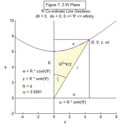In this context ψ can be called "the hyperbolic angle" of the projection.

Three-Dimensional Representations of Curvature

Hypersurface with Positive Curvature

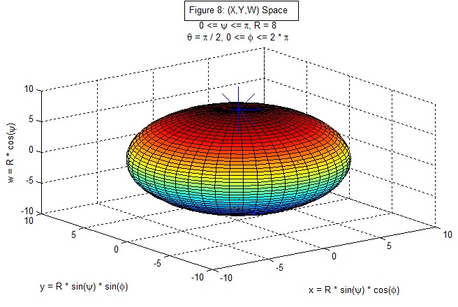
Figure 8: (X, Y, W) space, with θ = π/2, cos(θ) = 0, sin(θ) = 1, z = 0, north pole (NP) of the two-dimensional surface (sphere) at (0, 0, 0, R).
The arc length along a ψ geodesic (φ fixed, dφ = 0) from the NP to a point = r = R * ψ.

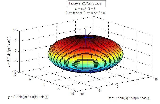
Figure 9: (X, Y, Z) space, with ψ = π/2, cos(ψ) = 0, sin(ψ) = 1, w = 0, NP at (0, 0, R, 0).
The arc length along a θ geodesic (φ fixed, dφ = 0) from the NP to a point = r = R * θ.

Hypersurface with Negative Curvature

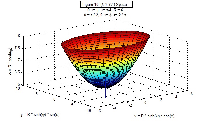
Figure 10: (X, Y, W) space, with θ = π/2, cos(θ) = 0, sin(θ) = 1, z = 0, pole of the two-dimensional surface at (0, 0, 0, R).
The arc length along a ψ geodesic (φ fixed, dφ = 0) from the pole to the point = s = R * ∫₀^ψ'(cosh²ψ + sinh²ψ)^1/2dψ.

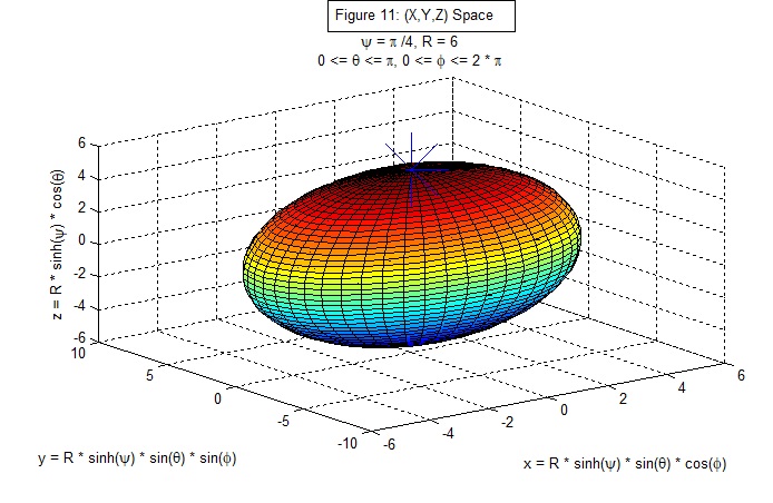
Figure 11: (X, Y, Z) space, with ψ = pi/4, cosh(ψ) = 1.32, sinh(ψ) = 0.87, w = 7.95, z = 5.21, pole at (0, 0, 5.21, 7.95).
The arc length along a θ geodesic (φ fixed, dφ = 0) from the NP to a point = s = R * sinh(ψ) * θ.

Alternative Parametrizations of the Metrics

Let dΩ² = dθ² + sin²(θ) dφ², 0 <= θ <= π, 0 <= φ <= 2π.

Zero Curvature

dl² = R² (dψ² + ψ² dΩ²), let χ = ψ, then dl² = R² (dχ² + χ² dΩ²). Let χ = ψ = r / R, → dl² = dr² + r² dΩ², 0 <= r < ∞.

Positive Curvature

dl² = R² (dψ² + sin²(ψ) dΩ²), let χ = sin(ψ) ∈ [0, 1], dχ = cos(ψ)dψ, → dχ² = cos²(ψ)dψ² = (1 – sin²(ψ) dΨ², and
      dψ² = dχ² / (1 – sin²(ψ)) = dχ² / (1 – χ²). Then dl² = R² ( dχ² / (1 – χ²) + χ² dΩ² ).

Let dr² = R² dχ²/ (1 - χ²) → dr / R = dχ / sqrt(1 - χ²) → r / R = sin^-1(χ) → χ = sin(r/R) → dl² = dr² + R² (r/R) dΩ², r = R ψ, 0 <= ψ <= π.

Negative Curvature

dl² = R² (dψ² + sinh²(ψ) dΩ²), let χ = sinh(ψ) ∈ [0, ∞), dχ = cosh(ψ)dψ, dχ² = cosh²(ψ)dψ² = (1 + sinh²(ψ) dψ², and
dψ² = dχ² / (1 + sinh²(ψ)) = dχ² / (1 + χ²). Then dl² = R² (dχ² / (1 + χ²) + χ² dΩ²).

Let dr² = R² dχ²/ (1 + χ²) → dr / R = dχ / sqrt(1+ χ²) → r / R = sinh^-1(χ) → χ = sinh(r/R) Then dl² = dr² + R² sinh²(r/R) dΩ², r = R ψ, 0 <= ψ < ∞.

Compact Form

dl² = dr² + Sκ(r) dΩ²

Sκ(r) = R sin(r/R) Sκ(r) = r Sκ(r) = R sinh(r/R)

(κ = +1) (κ = 0) (κ = -1)

0 <= r < ∞ r = R ψ, 0 <= ψ <= π r = R ψ, 0 <= ψ < ∞

Standard Model

In a universe with radiation (r), matter (m), and a cosmological constant (Λ) components, the Friedmann equation can be written as:

                H² / H0² = Ω⁰_r / a⁴ + Ω⁰_m / a³ + Ω⁰_Λ + (1 – Ω⁰) / a²,

where a = scale factor, H(t) = (da/dt) / a, H0 = H(t₀), t₀ = present time, and Ω⁰_r, Ω⁰_m, and Ω⁰_Λ, are the density parameters at t = t₀.

The total density of the components is Ω⁰ = Ω⁰_r + Ω⁰_m + Ω⁰_Λ. The curvature parameter Κ = -1, 0, 1 as Ω⁰ <, =, > 1.

The solution of the Friedmann equation provides a relation between the scale factor a and time t.

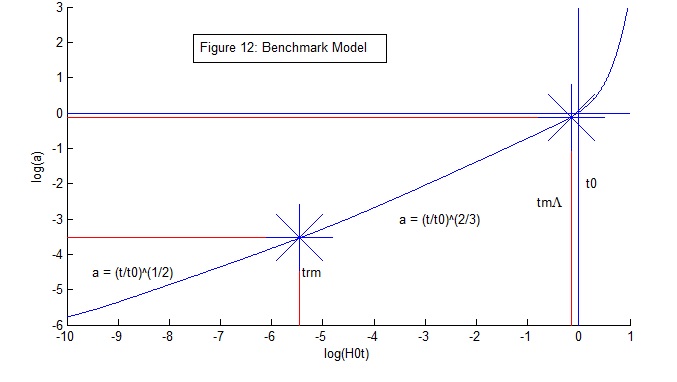
Figure 12: Model densities: Ω⁰_r = 9*10^-9, Ω⁰_m = 0.31, Ω⁰_Λ = Ω_Λ = 0.69.

Radiation-matter equality, a_rm = 2.9*10^-4 (Z = 3447), t_rm = 0.05 Myr; matter-Λ equality, a_mΛ = 0.77 (Z = 0.2987), t_mΛ = 10.2 Gyr, a(t₀) = 1.

Model Universes – Matter and Curvature

With matter as the only component of the universe, matter’s density, Ω⁰_m = Ω⁰, determines the universe’s evolution.

The Friedmann equation can be written as: (da/dt)² / H0² = Ω⁰ / a + (1 - Ω⁰).

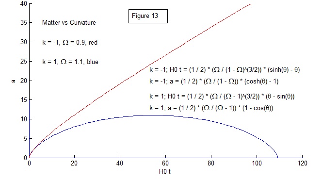
Figure 13: If Ω⁰ > 1, the universe is positively curved and collapses into a “Big Crunch.” Conversely, if Ω⁰ < 0, the universe is negatively curved and expands forever in a “Big Chill.”

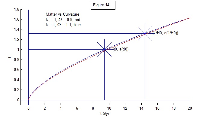
Figure 14: The two trajectories only diverge significantly at a time greater than t = 1 / H0 = 14.4 Gyrs.

References

Komissarov, S.S. (2002). Cosmology. Retrieved March 1 2018, from https://www1.maths.leeds.ac.uk/~serguei/teaching/cosmology.pdf.

Morgan, F. (1998). Riemannian Geometry: A Beginners Guide. Natick, Mass.: Peters.

Narlikar, J.V. (2002). An Introduction to Cosmology (3rd ed.). Cambridge: Cambridge UP.

Ryden, B. (2017). Introduction to Cosmology (2nd ed.). Cambridge: Cambridge UP.

Scott, Douglas (2018). Astronomy 403: Cosmology. University of British Columbia Course Notes.

Thomas, G.B. Jr. (1960). Calculus and Analytic Geometry. Don Mills, Ontario: Addison-Wesley.

See Also:

Wikipedia (2024, April 24). Dark Matter.

Wikipedia (2024, April 24). Dark Energy.

Wikipedia (2024, April 24). Shape of the Universe.

Wikepedia (2024, April 24). Expansion of the Universe.

Wikepedia (2024, May 7). Hyperbolic Angle.